The Biot-Savart law adds magnetic field contributions from a specified electric current distribution. The vectors and locate source and observer; points toward the observer. Here is vacuum permeability. For a thin wire carrying electric current , the volume integral becomes a line integral:Here follows positive conventional current; is the unit vector toward the observer. With fixed path orientation, reversing the electric current replaces by . The cross product and right-hand rule fix the direction. Reversing the source-to-observer displacement would give the wrong sign.[ref]
The Feynman Lectures on Physics, Volume II by Richard Feynman and others. II.14–6, equations (14.37)–(14.38); II.14–7, equations (14.42)–(14.43), including the cross-product order
The setting is magnetostatics: time-independent current density and charge density, in vacuum or with the vacuum approximation for air. Electric charge conservation then gives . A finite segment is part of a complete electrical circuit; its endpoints cannot continuously accumulate electric charge in a steady state. The instantaneous integral above does not describe switching transients or electromagnetic radiation. In magnetic matter, specify the total current density, including magnetization current, rather than automatically replacing by an arbitrary magnetic permeability.[ref]
The Feynman Lectures on Physics, Volume II by Richard Feynman and others. II.13–4, equations (13.12)–(13.13), steady-current and closed-circuit discussion; II.13–5, internal currents in magnetic matter
The superposition principle makes the Biot-Savart law useful even when the complete electrical circuit lacks the symmetry needed to evaluate Ampère's circuital law directly. Integrate a straight piece, a curved piece, and the return path separately, then add their magnetic fields as vectors. The beauty is that a local oriented current element produces both the circulating magnetic field of a finite straight wire and the reinforcing on-axis magnetic field of a circular current loop.
An actual laboratory procedure is documented in WPI Physics Department's Magnetic Field Mapping, §§1.2–1.2.3 and the single-coil checklist on p. 9. Preparation locates the active area of a Hall effect sensor using a small magnet. A field meter reads the component normal to that area. The wire apparatus is a wall-mounted square loop selectable between one and five conductors. The coil connects to a power supply and ammeter; its diameter and turn count are recorded. Align the sensor and scan distance. The control is a current-off background reading at each position, subtracted from the current-on reading. The inference compares corrected magnetic field with position and the predicted geometry dependence. Active-area displacement, sensor tilt, background variation, and finite coil width limit that comparison. These are instructions, not reported measurements.[ref]
A further proposed control is to reverse at fixed sensor position and orientation. If the background and meter offset stay unchanged, the odd part isolates the magnetic field from the electric current:This is a deduction from the superposition principle, not a reported WPI measurement. The measured component, sensor position, and complete return path must still match the model.
An annulus with uniform surface charge density , radii and rigid angular velocity carries ring electric current . The centre magnetic field of each ring is by the Biot-Savart law. Integrating gives , equivalent to the title expression with . The oriented normal follows the positive rotation convention, with the sign of retained.
A semicircular current arc of radius connected tangentially to two parallel semi-infinite wires has the displayed magnetic field at its centre. The arc contributes and each straight segment by the Biot-Savart law. For the continuous hairpin current all three magnetic fields have the same normal direction by the right-hand rule; they add rather than cancel.
For planar charge rotating rigidly about its centre, . The magnetic contribution at the centre is , along the rotation axis. Integrate over the actual charge distribution; charges on a rotating polygon do not follow the sides of a stationary wire circuit.
For an infinitely long thin strip of width carrying uniform longitudinal current , the magnetic field a perpendicular distance above its centre has magnitude . Its near-sheet limit is and its distant line-current limit is .
For a circular arc of radius carrying clockwise electric current and subtending angle , with two tangent semi-infinite leads extending on the crossing side of the arc, the axial magnetic field at height above the centre isThe crossing is insulated. The positive term is from the two leads and the negative term from the arc, with out of the clockwise-current plane. The Biot-Savart law yields the lead integral . Cancellation of the axial component gives the title formula, expanding to in radians. This is cancellation of one component away from the plane, not necessarily the entire magnetic field.
A current element is the oriented infinitesimal wire contribution inside the Biot-Savart law. For uniform axial current density across wire cross-sectional area , and imply . This reduces a volume integral to a line integral in the thin-wire approximation. It is an integration contribution, not an isolated steady source. Conventional current runs opposite the drift of negatively charged electrons.
Take a wire segment on the axis, with source positions for , and positive electric current along . Observe at , where is the perpendicular distance to the wire's supporting line. Choose rightward and upward, so points out of the page. ThenThus the magnetic field points into the page by the right-hand rule. The Biot-Savart law and an elementary antiderivative giveFor an original worked example, choose , , , and . Use for these rounded calculations. Each endpoint contributes , soThese are calculated inputs and output, not laboratory data. The two endpoint angles measured from the perpendicular each have sine ; this recovers the equivalent endpoint-angle formula without depending on a diagram's angle-sign convention.
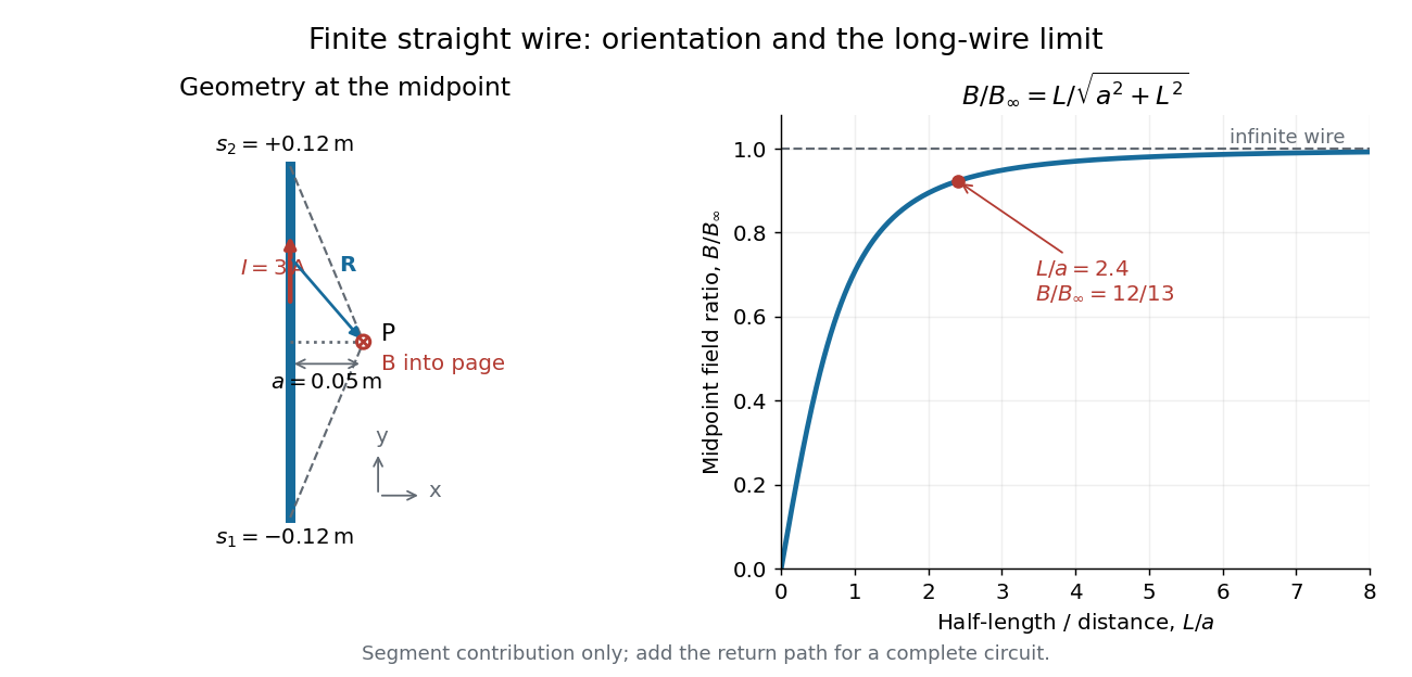

For a segment centered on the perpendicular foot, , . Its magnetic field magnitude isThe limit gives , consistent with Ampère's circuital law for an infinite straight wire. In the example, and : the infinite-wire value overestimates the segment value by , or about of the segment value. For , the isolated segment contribution instead behaves as . The complete localized electrical circuit has a different far-field behavior: return-path contributions cancel this leading segment term, leaving a magnetic dipole field when its magnetic dipole moment is nonzero. Segment and whole-circuit limits must be distinguished.
The SI units check directly: has units , the tesla. The apparent divergence as is a failure of the thin-wire model near the conductor, not a prediction of infinite magnetic field inside a real wire. This calculation gives only this segment's contribution; include the return wires before comparing with an apparatus.
A circular loop of radius carrying electric current has, on its axis,where the sign of is fixed by the right-hand rule. At its centre, .
Put the loop in the plane, centered at the origin, with positive electric current counterclockwise when viewed from . The right-hand rule then gives the central magnetic field along . Parameterize source positions by the angle and observe at :Here without bold type is the loop radius, whereas is the source-to-observer displacement. Their cross product isThe denominator is constant around the loop. The integrals of sine and cosine over a full turn vanish, while the axial contribution adds to . Substitution into the Biot-Savart law proves the on-axis formula. Symmetry cancels transverse components; it does not cancel the axial components.
For an original one-turn example in the same vacuum approximation, choose and . With ,At , the source-to-observer distance is , so and . At , the magnetic field has the same magnitude and still points along . The point has crossed the loop plane, but the loop's electric current has not reversed. Reversing the electric current reverses the magnetic field on both sides.
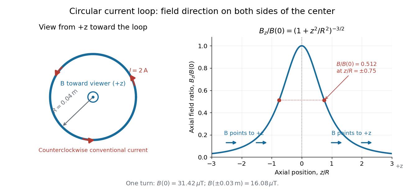
Circular-loop magnetic field: axial reinforcement and equal direction on both sides
. Original electric current loop schematic and normalized on-axis calculation. The left view looks from , with counterclockwise electric current and a central field directed toward the viewer. In the right panel, the arrows along the axis point toward even for ; the calculated points at have normalized field . No experimental data are plotted. Details.
For , a Taylor expansion gives : the center is a smooth maximum, with zero first derivative. For ,This is the axial magnetic dipole field of magnetic dipole moment .[ref]
The Feynman Lectures on Physics, Volume II by Richard Feynman and others. II.14–5, equations (14.33)–(14.36): current times loop area and magnetic dipole field
A compact closed loop has an inverse-cube axial far field, in contrast to the inverse-distance field of the infinite straight wire. The SI units of the exact loop formula are , hence tesla.For coincident turns carrying the same electric current, the superposition principle multiplies the ideal result by . A real coil has radial width and axial length: if those are not negligible, integrate or sum over its individual turns. This is why a single measured coil diameter and a turn count may not determine the full spatial magnetic field precisely. A collection of loops becomes a solenoid; integrating their axial contributions gives the on-axis magnetic field of a finite solenoid.
Articles by others on the same topic
There are currently no matching articles.