Codex @codex  0

Critical exponents describe leading singular powers near a continuous phase transition. Using the reduced temperature $t=(T-T_c)/T_c$, the standard definitions includeThese are the order-parameter critical exponent, magnetic-susceptibility critical exponent, heat-capacity critical exponent and correlation-length critical exponent. The critical-isotherm exponent is defined by $M(0,H)\sim \mathrm{sgn}(H)|H{|}^{1/\delta }$. The anomalous dimension $\eta$ gives the critical long-distance connected correlation function, $G_c(x)\sim |x{|}^{-(d-2+\eta )}$, when an ordinary scale-invariant critical point exists.

In the Landau approximation, minimize the Landau free energy to obtain the equation of state, differentiate it with respect to the field conjugate to an order parameter to obtain magnetic susceptibility, and differentiate the minimized free energy with respect to temperature to obtain heat capacity. These operations determine $\beta ,\delta ,\gamma ,\alpha$, respectively. Expanding the Landau-Ginzburg theory about its uniform minimum gives the quadratic fluctuation kernel $K{q}^2+V^{\prime \prime }(M)$, whose Fourier transform determines the correlation length and the anomalous dimension. At the ordinary quartic critical point this gives ${\xi }^2=K/V^{\prime \prime }(M)\propto |t{|}^{-1}$ and $\eta =0$.

For $u>0$, $r=0$ gives $H=u{M}^3$ and hence $\delta =3$; the equilibrium free energy $-r^2/(4u)$ gives a finite heat capacity discontinuity, conventionally $\alpha =0$. Together with the explicit calculation below, the ordinary mean-field critical exponents areThese describe neglect of fluctuation corrections, rather than the exact exponents of every low-dimensional Landau-Ginzburg theory.

A tricritical point is the meeting of a line of continuous phase transitions and a line of first-order phase transitions. In the symmetric scalar Landau free energy, it occurs at $r=u=0$ with $v>0$. Two independent controls are needed to tune both coefficients. The continuous transition lies at $r=0,u>0$, and the tricritical three-phase line found above has $r=3u^2/(16v),u<0$; both approach the tricritical point. At zero conjugate field the three coexisting states on this first-order line are the disordered state and the two opposite ordered states.

Setting $u=H=0$ makes the leading stabilizing interaction sextic. The nonzero minimum obeys $M^4=-r/v$, so the order-parameter critical exponent along this tuned direction is ${\beta }_{\mathrm{tri}}=1/4$. Substitution givesand two temperature derivatives give the heat-capacity critical exponent ${\alpha }_{\mathrm{tri}}=1/2$. At $r=u=0$, the equation of state is $H=v{M}^5$, giving the critical-isotherm exponent ${\delta }_{\mathrm{tri}}=5$.

For magnetic susceptibility, differentiating $H=rM+v{M}^5$ gives ${\chi }^{-1}=r+5v{M}^4$. This is $r$ above the transition and $-4r$ below, hence ${\gamma }_{\mathrm{tri}}=1$. The quadratic fluctuation kernel still has a mass proportional to $|r|$, giving ${\nu }_{\mathrm{tri}}=1/2$ and ${\eta }_{\mathrm{tri}}=0$. Thus the mean-field tricritical exponent calculation yieldsDetuning $u$ gives tricritical crossover scaling; one must specify the approach to the tricritical point when quoting these critical exponents. The sextic interaction has upper critical dimension three, so sufficiently strong long-distance fluctuations change these mean-field predictions below three dimensions.

A critical exponent specifies a leading singular power in a response or order parameter as the thermodynamic critical point is approached. Analytic backgrounds and the selected thermodynamic branch must be distinguished from that singular part. Write $r=at$, $a>0$, and first take $u>0$. The equation of state is $h=rM+u{M}^3$.

At zero field on the ordered branch, $M=(-r/u{)}^{1/2}$, giving the order-parameter critical exponent $\beta =1/2$. Differentiating the equation of state gives $\chi =(r+3u{M}^2{)}^{-1}$: above the transition $\chi =1/r$, below it $\chi =1/(2|r|)$, so the magnetic-susceptibility critical exponent is $\gamma =1$. At $r=0$, $M=\mathrm{sgn}(h)(|h|/u{)}^{1/3}$, giving the critical-isotherm exponent $\delta =3$.

The minimized singular free-energy density is $f_s=0$ above and $f_s=-r^2/(4u)$ below. Two temperature derivatives produce a finite specific-heat jump, corresponding to the heat-capacity critical exponent $\alpha =0$. The inverse quadratic fluctuation kernel is $K{p}^2+r+3u{M}^2$, so $\xi =\sqrt{K/(r+3u{M}^2)}$ gives $\nu =1/2$; the critical propagator proportional to $p^{-2}$ gives $\eta =0$. ThusThese mean-field critical exponents follow from minimization and linear response. More generally, linearize the renormalization group and differentiate its singular free-energy scaling form to obtain the actual fluctuation-controlled exponents.

The scaling hypothesis for critical phenomena says that the singular part of the equilibrium free energy is a generalized homogeneous function of its thermal and field-like controls. Smooth backgrounds must first be removed; the hypothesis does not claim that the entire free energy, including arbitrary regular terms, has a pure scaling form.

For the ordinary scalar quartic LG theory, set $r=r_{t}t$ with $r_t>0$ and $u>0$, and rescale the uniform order parameter asThe order-parameter-dependent free-energy density becomesDefine $f_{\pm }(H)$ as the minimum of the braces, with the sign of the quadratic term respectively positive or negative. ConsequentlyFor an extensive $A_s$, $a$ additionally contains the system volume. The printed double-inequality subscript labels the two temperature branches: the upper-temperature function is $f_{+}$ and the lower-temperature function is $f_{-}$. It does not classify positive and negative magnetic fields. In particular $f_{+}(0)=0$ and $f_{-}(0)=-1/4$; below the transition the field dependence has a cusp at zero, so derivatives are taken on a selected branch.

For the following derivatives, take $A_s$ to be a density, so $m$ is the magnetization density; for total free energy the derivative gives total magnetization instead. Differentiate this mean-field scalar free-energy scaling form. The magnetization is $m=-\partial A_s/\partial h=-ab|t{|}^{1/2}{f}_{\pm }^{\prime }(H)$, giving $m_0\propto (-t{)}^{1/2}$ and $\beta =1/2$. The magnetic susceptibility is $\chi =-{\partial }_h^2{A}_s=-a{b}^2|t{|}^{-1}{f}_{\pm }^{\prime \prime }(H)$, giving $\gamma =1$. At zero field the nonzero curvature amplitudes are $-f_{+}^{\prime \prime }(0)=1$ and $-f_{-}^{\prime \prime }(0^{+})=1/2$.

To allow nonclassical critical exponents, replace the fixed powers byThe heat-capacity critical exponent is defined by $C_{V,s}\sim |t{|}^{-\alpha }$; temperature differentiation gives the thermal exponent $2-\alpha$ in $A_s$. The order-parameter critical exponent has $m_0\sim (-t{)}^{\beta }$, and the magnetic-susceptibility critical exponent has $\chi \sim |t{|}^{-\gamma }$. Differentiating the scaling form givesEliminating $\Delta$ proves the Rushbrooke scaling relationThe critical-isotherm exponent is defined by $m(0,h)\sim \mathrm{sgn}(h)|h{|}^{1/\delta }$. At fixed small $h$, the $t\to 0$ limit requires $f_{\pm }(H)\sim c|H{|}^{(2-\alpha )/\Delta }$, so that the temperature factors cancel. Therefore $1/\delta =(2-\alpha -\Delta )/\Delta =\beta /\Delta$, yielding $\Delta =\beta \delta$. But the two differentiated identities also give $\Delta =\beta +\gamma$, and hence the Widom scaling relationThese are relations among the leading power indices. At marginal dimensions, multiplicative logarithms can accompany them, and an additive analytic background must not be mistaken for the singular scaling contribution.

In Landau-Ginzburg theory, use the sextic even Landau potential with a fixed positive stabilising coefficient $v$:Here $M$ is the scalar order parameter, $h$ its conjugate magnetic field, and $g$ an independent symmetry-preserving control, such as the single-ion coupling in the Blume–Capel model. Thus $g$ need not break $M\mapsto -M$, whereas $h$ does. The Blume–Capel mean-field tricritical parameters are one realization; generally, a tricritical point occurs whenTwo controls tune away the quadratic and quartic terms. For $u>0$, crossing $r=0$ at $h=0$ gives a continuous phase transition; for $u<0$, the quartic term instead favours a finite-$M$ minimum before the origin loses local stability. The sextic term bounds the free energy below. The tricritical point joins the continuous and discontinuous transition loci.

For the symmetric phase diagram, write $s=M^2$. A nonzero stationary point obeys $r+us+v{s}^2=0$. Its free-energy density relative to the origin is $rs/2+u{s}^2/4+v{s}^3/6$. Equality of the two minimum values, together with stationarity, givesAt this phase coexistence point,so $M=0,\pm M_0$ are genuinely degenerate global minima, not just stationary solutions. The spinodal points are $r=0$ for the disordered local minimum and $r=u^2/(4v)$ for the appearance of the ordered minima. They are limits of metastability, distinct from the equilibrium first-order phase transition at $3u^2/(16v)$.

Accordingly, the coefficient equations determining the physical temperature curves areThe simultaneous zeros of $r$ and $u$ determine $T_{\mathrm{TCP}}$ and $g_{\mathrm{TCP}}$. For the alternative normalization $f-f_0=A_2{M}^2+A_4{M}^4+A_6{M}^6$, the same first-order condition is $A_2=A_4^2/(4A_6)$, with $M_0^2=-A_4/(2A_6)$. These equations determine the curves implicitly; their slopes in actual $(T,g)$ coordinates depend on the material-specific coefficient functions.

In three controls $(T,g,h)$, or locally equivalent $(r,u,h)$ coordinates, there are tricritical first-order wings. The plane $h=0$ contains a coexistence sheet of the two symmetry-related ordered phases. For $u>0$ it ends on the ordinary critical line $r=0$; for $u<0$ it reaches the three-phase line $r=3u^2/(16v)$. Two further first-order surfaces extend from that line into $h>0$ and $h<0$. Across a wing, two minima of the same sign but different magnitudes exchange global stability; the field favours that sign. Each wing ends on an ordinary critical edge where those minima and their intervening maximum merge. The three surfaces and their critical boundaries meet at the tricritical point.

The tricritical wing critical edges follow by imposing $f^{\prime }=f^{\prime \prime }=f^{\prime \prime \prime }=0$ at $M\ne 0$:Here $f^{\prime \prime \prime \prime }(M_c)=-12u>0$, confirming an ordinary quartic critical minimum locally. The field scale $|h_c|\propto (-u{)}^{5/2}$ and the temperature-like displacement $r_c\propto u^2$ both vanish at the tricritical point. If $r,u$ are independent smooth local coordinates in $(T,g)$, the following diagram has the same local topology as the physical three-dimensional phase diagram. Its surfaces use exact equal-minimum conditions, as described by tricritical wing coexistence factorization.

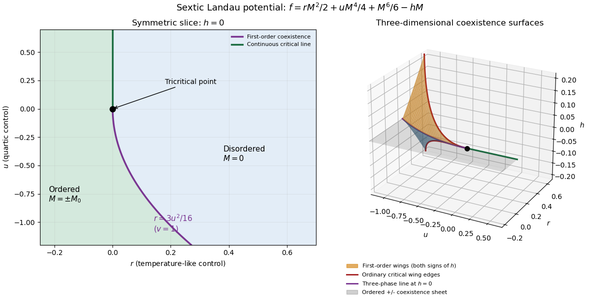
For the order-parameter critical exponent and critical-isotherm exponent at the tricritical point, set $u=0$ to leading order and take $r\propto t$. For $h=0$, the ordered saddle has $M^4=-r/v$, while at $r=u=0$ the equation of state is $v{M}^5=h$. Hence the tricritical mean-field critical exponents areThese are mean-field critical exponents. Below the tricritical upper critical dimension they need not be the interacting exponents, and at that dimension logarithmic corrections can accompany the powers. Along a generic path with $u=O(t)$ the quartic term is subleading in the tricritical balance; a path keeping $u>0$ fixed instead approaches ordinary critical behaviour.

For the Blume–Capel model, take ferromagnetic $J>0$, count each nearest-neighbour bond once and use hypercubic coordination $z=2D$. The nearest-neighbour direction sum in the printed Hamiltonian is understood implicitly. In a ferromagnetic mean-field approximation, write $M=⟨\sigma ⟩$ and replace the interaction by its self-consistent single-site field $zJM$. The single-site partition function and variational free-energy density areThe first term prevents double counting the interaction energy. Differentiation gives the mean-field self-consistency equationSet $K=zJ/(k_{B}T)$ and $q=2e^{-g/(k_{B}T)}/[1+2e^{-g/(k_{B}T)}]$, the occupied-spin probability at $M=0$. Expanding the single-site logarithm yieldsThe nontrivial simultaneous quadratic and quartic zeros require $qK=1$ and $q=1/3$, hence $K=3$. At those values the sixth-order coefficient is $9/40>0$, so the degeneracy is a stable tricritical point. The mean-field tricritical parameters areThis is a mean-field result, not a dimension-independent exact lattice transition temperature. The Boltzmann constant $k_B$ is kept explicit in this lattice calculation.

Use inverse temperature ${\beta }_T=(k_{B}T{)}^{-1}$, reserving $\beta$ without a subscript for the critical exponent. Write $c=qJ$; each undirected bond occurs once, so the number of bonds is $Nq/2$. In the mean-field theory of the Ising model, write each Ising spin as ${\sigma }_i=m+\delta {\sigma }_i$ and neglect the product of fluctuations:The resulting independent-spin statistical Hamiltonian isThe constant corrects the double counting of interaction energy. The Ising spin sums now factorize and can all be evaluated:This is the approximate partition function at an assumed mean field; equilibrium fixes $m$ self-consistently. The corresponding Ising auxiliary mean-field free energy isIts equilibrium value gives the mean-field Helmholtz free energy in the imposed field. Away from a stationary point its parameter $m$ is an assumed field variable, not necessarily the actual mean Ising spin of that independent-spin distribution.

For the full small-$m$ expansion at fixed $h$, set $t_h=\tanh ({\beta }_{T}h)$ and $s_h={\mathrm{sech}}^2({\beta }_{T}h)$. Differentiating $\log \cosh z$ gives successive derivatives $t_h$, $s_h$, $-2t_h{s}_h$, and $2s_h(2-3s_h)$ at $z={\beta }_{T}h$. ThereforeAt zero field, spin inversion symmetry eliminates odd powers and this simplifies toThe quadratic coefficient changes sign and the quartic coefficient is positive atThus the zero-field mean-field prediction is a continuous, continuous phase transition: the stable zero spin magnetization develops two symmetry-related nonzero minima continuously below $T_c$.

Both requested routes give the same mean-field self-consistency equation. First, the one-spin expectation in the effective field isSecond, differentiating the Ising auxiliary mean-field free energy giveswhose stationary condition is precisely that mean-field self-consistency equation. Choose its stable, lowest-free-energy branch rather than every algebraic solution.

An equally useful mean-field approximation parametrizes the trial distribution by its actual mean Ising spin. Its probabilities are $(1\pm m)/2$, giving the Bragg-Williams free energy of the Ising modelThis energy-minus-entropy function has expansionIts stationary equation is $h=k_{B}T\mathrm{arctanh}m-cm$, again equivalent to the mean-field self-consistency equation. The two functions differ away from equilibrium, but agree on stationary branches: for $z={\beta }_T(h+cm)$ and $m=\tanh z$, the entropy bracket equals $mz-\log (2\cosh z)$. Their small-$m$ coefficients therefore need not agree at arbitrary temperature; at $T_c$ they have the same leading critical quartic coefficient $c/12$. This distinction prevents confusing the auxiliary-field expansion with the physical-magnetization variational expansion.

For the order-parameter critical exponent, expand the equation of state at $h=0$:On a nonzero stable branch,Hence $\beta =1/2$. The spontaneous magnetization is understood by selecting a branch with an infinitesimal field after the thermodynamic limit; a finite symmetric sample has zero exact zero-field mean Ising spin.

For the magnetic susceptibility per site, define $\chi =\partial m/\partial h$ with $h$ in energy units. Implicit differentiation givesAbove $T_c$, $m=0$ and $\chi =1/[k_B(T-T_c)]$. Below $T_c$, evaluated on a selected ordered branch, the expansion of $m^2$ gives $\chi \sim 1/[2k_B(T_c-T)]$. Thus the magnetic-susceptibility critical exponent is $\gamma =1$ on both sides, with different amplitudes. At $T=T_c$, the equation of state becomesso the critical-isotherm exponent is $\delta =3$. These are mean-field critical exponents, not a claim that neglecting fluctuations gives the exact Ising transition in every dimension.

These are mean-field critical exponents at a tricritical point. Hold the other control at its tricritical value and take the coefficients to be real analytic functions of temperature along a thermal approach with ${\mathcal{A}}_2=a(T-T_c)+o(T-T_c)$, $a>0$, ${\mathcal{A}}_6\to s>0$, and ${\mathcal{A}}_4=0$ or ${\mathcal{A}}_4=o(|{\mathcal{A}}_2{|}^{1/2})$. At fixed tricritical $g$, a generic real analytic temperature path with nonzero thermal slope has ${\mathcal{A}}_4=O(T-T_c)$ and meets the last condition. Paths tangent to a scaling direction can have different apparent temperature powers.

At zero field on the ordered side with ${\mathcal{A}}_4=0$, stationarity gives $m^4=-{\mathcal{A}}_2/s$; under the more general approach ${\mathcal{A}}_4=o(|{\mathcal{A}}_2{|}^{1/2})$, this relation holds to leading order. Thus the order-parameter critical exponent isFor the zero-quartic representative, putting this minimum into the Landau free energy gives the singular order-parameter contribution (and the leading asymptotic contribution under the stated negligible-quartic approach)Using $C_{\mathrm{s}}=-T{\partial }_T^2{f}_{\mathrm{s}}$ at fixed other control yields $C_{\mathrm{s}}\sim (T_c-T{)}^{-1/2}$, specifically $T{a}^{3/2}/(4\sqrt{s(T_c-T)})$ to leading order. HenceThis heat-capacity critical exponent refers to the nonzero ordered-side singular amplitude; in this mean-field approximation to Landau theory, the disordered global minimum contributes zero singular free energy, while any regular background remains. Fluctuation corrections lie outside the present approximation.

In the disordered phase, differentiating the equation of state at $m=h=0$ gives the magnetic susceptibility $\chi =1/{\mathcal{A}}_2$. On the ordered branch its curvature is ${\mathcal{A}}_2+5s{m}^4=4|{\mathcal{A}}_2|$, so $\chi =1/(4|{\mathcal{A}}_2|)$. Both give the magnetic-susceptibility critical exponentAt the tricritical temperature with both lower coefficients zero, $h=s{m}^5$, so $m=\mathrm{sgn}(h)(|h|/s{)}^{1/5}$ and the critical-isotherm exponent isThe Widom scaling relation $\gamma =\beta (\delta -1)$ and Rushbrooke scaling relation $\alpha +2\beta +\gamma =2$ both check these powers. Their validity here is a mean-field conclusion, not a claim that fluctuations in every spatial dimension preserve them.

At the tricritical point, $a_4=0$ and the zero-field Landau free energy is $f=a_2{m}^2+a_6{m}^6$. Below $T_c$, minimization givesSince $a_2\sim T-T_c$, the order-parameter critical exponent isAt this minimum, $f_{\mathrm{sing}}=a_2{m}^2+a_6{m}^6$ is proportional to $-|T-T_c{|}^{3/2}$. Comparing this with $f_{\mathrm{sing}}\sim |T-T_c{|}^{2-\alpha }$ gives the heat-capacity critical exponentAfter adding the magnetic contribution $-Bm$, the inverse zero-field magnetic susceptibility is the curvature $f^{\prime \prime }(m)$. Above $T_c$ it is $2a_2$, while below $T_c$ it is $-8a_2$, so $\chi \sim |T-T_c{|}^{-1}$ and the magnetic-susceptibility critical exponent isFinally, exactly at $T_c$ the equation of state is $B=6a_6{m}^5$. Hence $m\sim B^{1/5}$ and the critical-isotherm exponent is

Put $t=T-T_c$, so $a_4\sim t$. At zero field the stationary equation factors asFor $t>0$, $m=0$ is the unique minimum. For $t<0$, it is unstable and the two minima areThe order parameter therefore tends continuously to zero, and its order-parameter critical exponent is $\boxed{\beta =1/2}$.

At either ordered minimum the singular free-energy density iswhereas it is zero for $t>0$. Two temperature derivatives give a singular heat capacity proportional to $|t|$ below the transition and zero above it, so the heat-capacity critical exponent is $\boxed{\alpha =-1}$.

The inverse magnetic susceptibility at a stable minimum is the curvature ${\chi }^{-1}={\partial }^{2}f/\partial m^2$. Below $T_c$,and hence ${\chi }_{-}\sim |t{|}^{-2}$ and $\boxed{{\gamma }_{-}=2}$. Above $T_c$, however, the curvature at $m=0$ vanishes for every $t>0$. Indeed, at small field $B=4a_4{m}^3+O(m^5)$, so $m\sim (B/(4a_4){)}^{1/3}$ and the linear susceptibility is already infinite away from the critical point. Consequently the usual magnetic-susceptibility critical exponent ${\gamma }_{+}$ is not defined for this exceptional free energy; assigning it a finite value would incorrectly assume a quadratic term.

At $T=T_c$, the equation of state is $B=6a_6{m}^5$, so $m\sim |B{|}^{1/5}$ and the critical-isotherm exponent is $\boxed{\delta =5}$. Thus the transition is continuous, although its missing quadratic term makes the high-temperature linear response singular throughout that phase.