Thermodynamic limit

The thermodynamic limit describes a sequence of larger systems, not a single enormous specimen: particle number $N$ and volume $V$ tend to infinity with number density $n=N/V$ fixed. Hold the chosen intensive and extensive thermodynamic quantities such as temperature $T$ and an applied magnetic field fixed along that sequence. In the canonical ensemble the controls are $T,N,V$; in the grand canonical ensemble one instead fixes $T$ and chemical potential, and the limiting number density is a result, possibly with a jump at phase coexistence. These are different specifications of a limiting experiment.

The useful limit is usually an intensive and extensive thermodynamic quantities normalization of the Helmholtz free energy, not a finite limit of the total extensive quantity itself:Here $Z_{N,V}$ is the canonical partition function, $k_B$ is the Boltzmann constant, $f$ is free-energy density, and $a$ is Helmholtz free energy per particle. Thus $F_{N,V}=Vf+o(V)$ when the limit exists; finite systems need not be exactly extensive quantities because of the surface correction to thermodynamic free energy.

Specify the interactions and the growing containers too. For a conventional fluid, use a fixed stable pair potential with a tempered pair potential tail, and containers whose boundary layer of any fixed thickness occupies a vanishing fraction of the volume; uniformly enlarged cubes work, a tube of fixed cross-section does not give the same bulk limit. For a finite-range Ising model, keep the lattice spacing and bond coupling fixed while enlarging all intended spatial directions. Ordinary bounded wall interactions or periodic boundary conditions can then give the same bulk free-energy density, although boundary conditions can select different spontaneous symmetry breaking states. This is a set of hypotheses, not a theorem that every interaction has a boundary-independent limit.^[ref]

The Curie–Weiss model below deliberately uses a different limiting prescription: its all-to-all coupling is divided by $N$. Without that factor its interaction energy would grow as $N^2$, rather than as an extensive quantity. The model has no spatial wall or correlation length to compare with a container; it is an exactly summable illustration of finite-size rounding, not a quantitative model of the fluid experiment below.

For finitely many microstates with finite energies $E_{\alpha }(h)$ that are real analytic functions of a real control $h$, the canonical partition function at $T>0$ is a finite positive sum:It and the resulting Helmholtz free energy are locally real analytic functions of $T$ and $h$. Hence such a finite Ising model has no literal nonanalytic equilibrium phase transition. A limit of these real analytic functions can nevertheless fail to be a real analytic function; the narrow but smooth crossover can become a sharp phase transition.^[ref]

Finite particle number alone is not the hypothesis of a finite sum. Classical phase space is continuous, and a system of quantum states can have infinitely many energy eigenvalues: its partition function requires convergence and local bounds that permit differentiation or an analytic extension of the integral or thermal trace. A divergent partition function, a singularly changed statistical Hamiltonian, or the zero-temperature limit falls outside the finite-positive-sum argument. Observing a steep change in a finite sample therefore motivates a limiting model; it does not measure an actual infinity.

At zero field and with spin inversion symmetry in its boundary conditions, a finite Ising model pairs every configuration with its spin-reversed configuration. Their equal Boltzmann weights force the expected value of its spin magnetization $m=N^{-1}{\sum }_i{s}_i$ to vanish. Below a model's ordering critical temperature, an arbitrarily small positive field can instead select the positive spontaneous magnetization if size is taken to infinity first:The distinction is the order of limits and the stated symmetric boundary conditions; plus boundary conditions already break spin inversion symmetry. A zero-field symmetric mixture of the two ordered states can retain zero mean spin magnetization even in the thermodynamic limit. Also, $⟨|m|⟩>0$ in a finite system is not by itself proof of spontaneous symmetry breaking.^[ref]

Finite-size rounding replaces a limiting discontinuity or divergence by a finite crossover or peak. For a spatial system near a continuous phase transition, the bulk description ceases to apply unchanged when the correlation length becomes comparable with the sample size. How the crossover width and location depend on size also depends on the model, geometry and boundary conditions; there is no universal $1/N$ rule for every phase transition.

An exact finite example is the Curie–Weiss model with $s_i=\pm 1$, $J>0$, and a conjugate field $h$ in energy units. Set $K=J/(k_{B}T)$ and $u=h/(k_{B}T)$. Its statistical Hamiltonian and finite partition function areThe binomial coefficient counts the microstates with $k$ positive Ising spins. The diagonal terms in the square add a configuration-independent constant to the energy; retaining them fixes the normalization used here. Divide each summand by $Z_N$ to obtain the probability mass function of $m_k=(2k-N)/N$. In particular,The variance expression makes the finite response nonnegative, while spin inversion symmetry gives $⟨m⟩=0$ exactly at $u=0$ for every plotted $N$.

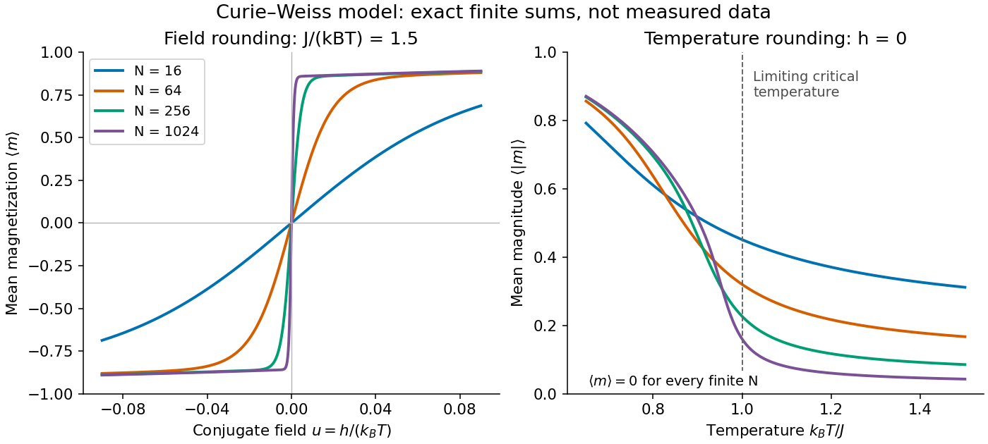
Every curve is computed from the finite partition function, without selecting one minimum of the Bragg-Williams free energy of the Ising model. The field panel holds $K=1.5$ fixed and shows increasingly rapid switching between opposite spin magnetizations. The temperature panel uses $u=0$: its nonzero $⟨|m|⟩$ measures the typical magnitude, while the mean spin magnetization stays zero. The reference $k_{B}T/J=1$ marks the limiting critical temperature, not a singular point of any finite curve.

A short limiting argument explains the field panel. Combining the binomial coefficient with its leading entropy gives a Helmholtz free energy per spin whose stationarity equation is $m=\tanh (Km+u)$. For $K>1$ and $u=0$ the two ordered minima have $m=\pm m_{\ast }$, where $m_{\ast }=\tanh (K{m}_{\ast })$. For large $N$ well below the critical temperature, their relative Boltzmann weight is approximately $e^{2Nu{m}_{\ast }}$, giving $⟨m⟩\approx m_{\ast }\tanh (Nu{m}_{\ast })$. Thus this two-peak approximation has a field width of order $1/(N{m}_{\ast })$ in $u$. It is not valid at the critical temperature, where the peaks merge; the figure uses the exact finite sum throughout.

For finite-range interactions and bounded wall couplings, only sites within an interaction range of the wall have altered local environments. In a regular container of linear size $L$ and dimension $d$, the surface area scales as $A\sim L^{d-1}$ while volume scales as $V\sim L^d$. A boundary contribution of order $A$ therefore gives an order-$1/L$ correction to free-energy density. Away from a critical phenomenon, a regular surface contribution often has the form $F=Vf+A\gamma +\cdots$, with $\gamma$ a wall Helmholtz free energy per area. Critical finite-size rounding, edges and long-range interactions require separate care; vanishing relative boundary size does not guarantee a simple surface expansion in every regime.

An exact check uses the zero-field nearest-neighbour Ising model on a chain of $N\ge 3$ sites with fixed coupling $J>0$ and $K=J/(k_{B}T)$. The open chain has $N-1$ bonds, while the periodic ring has $N$. Their finite partition functions and dimensionless Helmholtz free energies per spin $g_N=F_N/(N{k}_{B}T)$ areFor the open chain, sum the last Ising spin successively: each removed bond contributes $2\cosh K$, leaving a factor of two. For the ring, the transfer matrix for the one-dimensional Ising model has eigenvalues $2\cosh K$ and $2\sinh K$, and its $N$th power's trace gives the displayed sum. The two ends are a constant-size boundary in one dimension, so the open-chain total correction is $k_{B}T\log \cosh K$, and its per-spin correction is exactly proportional to $1/N$.

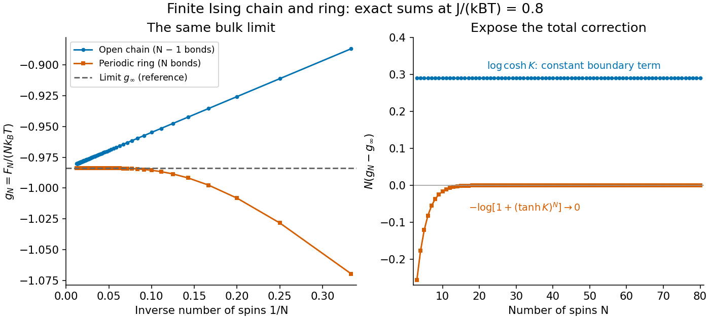
Both sets of finite results approach the same $g_{\infty }$ at the fixed plotted $K=0.8$. Multiplying the correction by $N$ exposes the open-chain boundary term, while the ring correction vanishes exponentially at fixed finite $K$. This model's thermodynamic limit remains a real analytic function at every positive temperature: having a thermodynamic limit does not require a phase transition.

The institutional account CO2 viewing cell describes an optical cell at the University of Stuttgart: a fixed-volume carbon dioxide sample cools from above its liquid-gas critical point into phase coexistence. The apparatus supplies a view through the cell and displayed temperature and pressure readings. Near roughly $31{}^{\circ }\mathrm{C}$, the account reports critical opalescence: enhanced scattering of light makes reflected light appear whitish and transmitted light dark. This readout reveals growing density thermal fluctuations; it is not a direct count of molecules or a measurement of an infinite correlation length. ^[ref]

Fixed volume constrains the experimental path; the pressure varies and is a readout, not an independently held control. The account explicitly identifies the clip as part of a longer cooldown and says its endpoints are not steady states. To test an equilibrium interpretation more closely, one would hold temperature until the readout settles, compare cooling and warming, and check optical background away from the liquid-gas critical point; these are proposed controls, not measurements reported on that page. The account does not provide cell dimensions, filling number density, calibration uncertainties or such control runs. The sample is finite: its striking appearance motivates the thermodynamic limit as a model of macroscopic sharpness, rather than demonstrating a literal equilibrium singularity.

Critical opalescence is enhanced scattering of light by large fluctuations near a thermodynamic critical point. The carbon-dioxide viewing-cell phase-transition experiment gives an observable finite-sample example; cloudiness alone does not establish a divergent correlation length.

A pair potential is stable when its total interaction energy obeys this lower bound for every allowed configuration, with a constant $B$ independent of $N$. It prevents collapse with an arbitrarily negative energy per particle. Stability alone does not control the long-distance contribution needed for the ordinary thermodynamic limit.

A standard sufficient tempering condition is this tail bound beyond a fixed radius, with $ϵ>0$ in spatial dimension $d$. It makes the distant interaction tail integrable; finite-range pair potentials satisfy it. Together with a stable pair potential and suitable growing containers, such assumptions support the conventional thermodynamic limit. A Curie–Weiss model with its size-dependent coupling uses a different prescription.