A muscular pump supporting blood circulation. Electrical activity, mechanical contraction and perception of heartbeat-related signals are distinguishable measurements.
A cardiac short axis is a transverse reference direction or imaging view relative to a specified cardiac long axis. For left-ventricular imaging, a short-axis plane is planned across the chamber rather than through its base-to-apex length. The chamber and anatomical landmarks must be specified; a patient's horizontal body plane is not automatically a cardiac short axis plane.
A primary cardiovascular magnetic resonance imaging protocol plans short-axis images using linked long-axis views and covers the ventricle from base to apex.[ref]
Standardized cardiovascular magnetic resonance imaging (CMR) protocols: 2020 update by Christopher M. Kramer and others. General techniques, Left ventricular structure and function; Figures 1–2
A cardiac short-axis stack turns successive cavity outlines into volumetric information.For an original geometrical construction, let be the unit vector along the chosen cardiac long axis. A transverse plane through satisfiesParallel planes at different axial positions sample different portions of the ventricle. With measured cavity areas and represented slice thicknesses , a simple volume estimate is .
An oblique slice also illustrates a useful caution. An ideal circular cylinder cut at angle away from its perpendicular section has an elliptical cross-sectional area . At this is about larger. This does not prove that an entire consistently acquired oblique stack overestimates volume: integrating all areas with the correct normal spacing and complete coverage still recovers volume. Orientation, spacing and coverage must be treated together. The major practical question is whether the chosen stack and image segmentation represent the complete intended cavity, not whether one slice happens to look circular.
A cardiac short-axis stack is a series of images across a cardiac chamber at successive positions approximately transverse to its cardiac long axis. In ventricular volumetry, the series must cover the intended cavity from its basal boundary toward the cardiac apex. A primary cardiovascular magnetic resonance imaging protocol specifies linked long-axis planning and short-axis coverage.[ref]
Standardized cardiovascular magnetic resonance imaging (CMR) protocols: 2020 update by Christopher M. Kramer and others. General techniques, Left ventricular structure and function; Figures 1–2
The stack supplies a spatial sum rather than a single diameter. Let be the segmented cavity area in slice at phase , and let be the represented distance along the stack normal. A basic approximation isAll areas in a given sum must refer to a compatible phase of the cardiac cycle. Image segmentation, slice coverage and phase matching are separate inputs to the volume estimate.
An original example uses four representative areas of 2, 6, 10 and 6 cm, each assigned 1 cm of axial extent. Their represented volume is 24 cm, or 24 mL. Omitting the basal 6 cm contribution reduces the result to 18 mL without changing the tracing quality of the other slices. If slice thickness is 0.8 cm but center spacing is 1 cm, the numerical integration convention must also account for the intervening extent; treating thickness and represented spacing as interchangeable changes the estimate.
Phase mixing causes a different error. An area from one slice near end-filling and another near end-ejection do not generally describe a cavity that existed at one time. A stack can therefore be complete spatially yet inconsistent temporally. With correctly matched phases, the derived end-diastolic volume and end-systolic volume can be used for stroke volume and ejection fraction; those formulas do not repair missing anatomy or mismatched acquisition phases.
Atrial contraction is active shortening of the atrial myocardium that contributes to moving blood from the atria into the ventricles. In the usual coordinated cardiac cycle, it occurs late in ventricular diastole, while the mitral valve and tricuspid valve permit filling. It supplements earlier passive filling; ventricular filling is not restricted to the period of atrial contraction.[ref]
For the left atrium, this active contribution is called atrial booster-pump function, distinguishable from atrial reservoir function and atrial conduit function. A volume balance separates storage from transport:where is summed pulmonary vein inflow and is net outflow through the mitral valve. During atrial contraction, a decrease in chamber volume can accompany outflow larger than the continuing inflow.
In an original example, the left atrium loses 15 mL during a chosen contraction interval while receiving 5 mL through the pulmonary veins. Integrating the balance shows that 20 mL must have left through the mitral valve. The volume decrease alone would undercount that interval's forward transport by 5 mL. Conversely, not all blood entering the left ventricle in that interval was necessarily stored before contraction began.
The distinction matters experimentally: a changing cavity volume, a velocity recorded at a valve and the trajectory of a particular parcel of blood are different observations. A primary flow-component study used time-resolved computed tomography, computational fluid dynamics and modeled particle paths to distinguish atrial transport routes.[ref]
Comprehensive left atrial flow component analysis reveals abnormal flow patterns in paroxysmal atrial fibrillation by Sophia Bäck and others. Abstract; Methods
A volume change associated with contraction is informative, but its interpretation requires the concurrent inflows and outflows.The apical impulse is a localized movement of the chest wall associated with the heart's mechanical activity, assessed by inspection or palpation. It is a surface observation rather than the anatomical cardiac apex itself. Its position, area, duration and timing within the cardiac cycle describe different features of the observation.
A primary study compared physical examination with two-dimensional echocardiography in 41 patients. The investigators found that impulse location relative to selected chest landmarks did not reliably identify increased left ventricular end-diastolic volume.[ref]
Accuracy of precordial palpation for detecting increased left ventricular volume by S. D. Eilen and others. Abstract, examination/echocardiography comparison and conclusion
The observation illustrates why an external landmark should be tested against an independent measurement instead of being treated as a direct cavity-volume reading. It does not establish a universal diagnostic rule for all patients.A simple original measurement model explains one source of ambiguity. Let represent an internal mechanical displacement and let the measured local surface displacement beThe coefficient summarizes an idealized mechanical coupling and viewing direction; represents other contributions. If the same internal motion mm is observed with or and zero background, the surface amplitudes are 1 mm and 0.5 mm. Changing the coupling can change the observed amplitude without changing the internal motion.
Real chest wall mechanics are more complicated than a single gain. The model nevertheless explains why body position, contact and the chosen observation site belong to the measurement description. Neither a surface displacement amplitude nor an apparent lateral position alone specifies ejection fraction or ventricular volume.
A cardiac long axis is a base-to-apex direction used to describe the heart or a specified ventricular chamber. In left-ventricular imaging it is commonly planned through the cardiac apex and the center of the mitral valve. It is a chamber-based anatomical reference, not necessarily the vertical direction of a patient's body or an image display.
The primary cardiovascular magnetic resonance imaging protocol specifies connected two-chamber, four-chamber and short-axis planning from anatomical landmarks.[ref]
Standardized cardiovascular magnetic resonance imaging (CMR) protocols: 2020 update by Christopher M. Kramer and others. General techniques, Left ventricular structure and function, items 3 and 6; Figures 1–3
A long-axis image plane contains the chosen cardiac long axis; the corresponding cardiac short axis describes a transverse direction or view. Different planes can contain the same long-axis line while displaying different walls and neighboring chambers.An original vector construction makes the distinction precise. Let be the apex position and a chosen basal reference point. Thenis the axial unit vector. A displacement has axial component and transverse component . The line alone does not determine how the transverse coordinates are rotated around it.
This geometry matters for cardiac image foreshortening. In a simple projection model, a length tilted by out of the display plane projects to . A 10 cm length tilted by appears about 8.66 cm long. This is a geometrical illustration, not a correction formula for a tomographic slice: a slice may miss the true apex rather than project it. Consistent landmark selection is therefore part of meaningful comparisons of cavity shape, motion and volume.
Cardiac image foreshortening occurs when a cardiac view represents a shorter apparent base-to-apex extent than the intended anatomical chamber length, often because the imaging plane misses the true cardiac apex. It can create an apparently thick false apex and affect derived ejection fraction and deformation measurements.
A primary echocardiography study acquired optimal and deliberately foreshortened views in 72 participants using a GE Vivid E9 system. The altered acquisition window was one rib-space above the optimal window; two analysis systems were used to compare derived quantities.[ref]
Impact of apical foreshortening on deformation measurements: a report from the EACVI-ASE Strain Standardization Task Force by Serkan Ünlü and others. Abstract, Aims and Methods and results
This tests acquisition geometry while keeping the participant the same, rather than interpreting every shorter-looking chamber as a biological change.An original ellipsoid model distinguishes a missed apex from a simple projected length. Letwith the true cardiac long axis along . The central long-axis plane includes both axial tips and has full length . A parallel offset plane instead intersects an ellipse whose apparent axial extent isAt , . A 10 cm true extent therefore appears as 8 cm in this model even though the slice was translated rather than rotated. Its apparent tips are not the original chamber tips.
This model is a geometrical explanation, not a clinical correction formula. A shorter outline can alter measured volume differently at end-diastolic volume and end-systolic volume; the ejection fraction error need not follow the length error by one fixed percentage. Consistent anatomical landmarks and independent views help distinguish actual chamber shape from the chosen section. Improving the repeatability of an outline inside an incorrect plane does not recover anatomy that was never acquired.
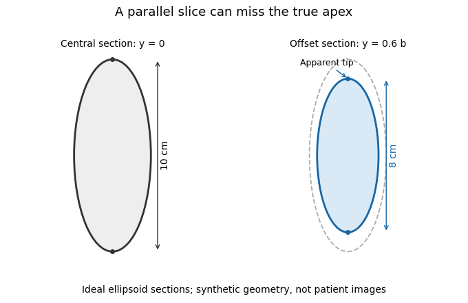
A parallel cardiac slice can miss the true apex
. Original sections of an ideal ellipsoid with axial semiaxis 5 cm and transverse semiaxis 2 cm. The central plane has full length 10 cm; a parallel plane offset by 0.6 times the transverse semiaxis has length 8 cm. Dashed outline shows the central section for comparison. Synthetic geometry, not patient data. Details.
Ejection fraction is the fraction of a ventricle's end-diastolic volume lost from its cavity during ejection:The numerator is volumetric stroke volume; is end-systolic volume. The chamber must be specified: right ventricular ejection fraction concerns the right ventricle, whereas a calculation for the left ventricle concerns its own pair of volumes.
Time-resolved magnetic resonance imaging can estimate the two volumes from a consistently defined cavity. A primary right-ventricular study used cine images and three-dimensional modelling in 120 subjects.[ref]
Reference right ventricular systolic and diastolic function normalized to age, gender and body surface area from steady-state free precession cardiovascular magnetic resonance by Alicia M. Maceira and others. Abstract, Methods and results
The ejection fraction is a derived quantity, not an additional independent volume observation.An original example illustrates its scale dependence. Volumes of 120 and 60 mL give and stroke volume 60 mL. Volumes of 240 and 120 mL give the same ejection fraction but twice the stroke volume. Consequently, ejection fraction alone does not determine cardiac output; heart rate and an appropriate forward-flow interpretation are also needed.
Its response to shared measurement errors is instructive. Multiplying both measured volumes by the same positive scale leaves the ejection fraction unchanged. Adding the same offset does not:For the 120/60 mL example, and mL change the calculated fraction from to , even though the volume difference remains 60 mL. This is an error-model example, not a universal correction for image segmentation. Likewise, cavity volume loss can include backward flow through a heart valve; the formula alone does not establish net useful delivery.
The chordae tendineae are collagen-rich tensile cords connecting valve leaflets of the mitral valve and tricuspid valve to papillary muscles. Their tension helps restrain the leaflets against displacement toward an atrium during ventricular systole. They are supports for pressure-loaded leaflets, rather than muscles that pull the valves open. The aortic valve and pulmonary valve do not have this chordal apparatus.[ref]
Anatomy and Physiology 2e by J. Gordon Betts and others. §19.1, Right Ventricle; Heart Valve Structure and Function
An original static model shows why the arrangement matters. Suppose a leaflet attachment experiences a resultant force from a pressure difference acting over effective area . Two equal tethers each carry tension at angle to the load axis. Their transverse components cancel and their axial components balance the load:A stipulated kPa over cm gives N. Changing from to raises each tether's tension from about to N without changing the pressure load.
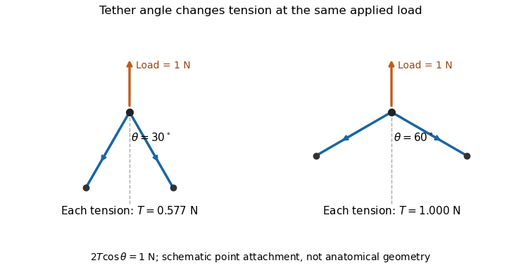

A primary experiment tested the related geometrical question in a left-heart simulator. Force transducers measured selected chordae tendineae while the positions of papillary muscles were changed. Different chordal types responded differently.[ref]
Effects of papillary muscle position on chordal force distribution: an in-vitro study by Jorge Hernan Jimenez and others. Abstract, Methods and Results
Real leaflets distribute loading among many attachments, so the two-tether model explains a mechanism without supplying a universal chordal force. Material behavior, geometry and the timing of ventricular contraction remain separate inputs.A papillary muscle is a muscular projection inside a ventricle that anchors chordae tendineae attached to the mitral valve or tricuspid valve. During ventricular systole, its contraction helps maintain the supporting geometry and tension that restrain the valve leaflets. Valve opening is driven by the appropriate pressure difference; a papillary muscle does not act as a cord-operated opener.[ref]
Anatomy and Physiology 2e by J. Gordon Betts and others. §19.1, Right Ventricle and Heart Valve Structure and Function
The anchor's position matters as well as its ability to contract. In a primary simulator study, investigators examined six human and five porcine specimens of the mitral valve, measuring six selected chordae tendineae with force transducers. Eight tested anchor configurations used 5 mm displacement components relative to a reference position. The resulting tension changes depended on which chord was measured.[ref] Moving an anchor therefore need not distribute extra load equally through the apparatus.
An original mechanical approximation illustrates the distinction. If a taut cord has reference length , cross-sectional area and effective Young's modulus , a small extra extension givesThis is a local Hooke's law approximation, not a claim that biological cords remain linear at every strain. Anchor displacement changes the cord's extension and direction, while active muscle contraction changes the moving support itself. In the equal-tether example under chordae tendineae, changing direction also changes the tension needed to balance a fixed leaflet load. The apparatus is consequently a coupled geometrical and muscular system; naming its parts alone does not predict its forces.
The cardiac apex is the pointed inferior end of the heart, formed mainly by the left ventricle. It lies toward the patient's left and supplies a useful endpoint for describing the cardiac long axis. The anterior interventricular sulcus and posterior interventricular sulcus approach this region along the ventricular surface.[ref]
The cardiac apex is an anatomical landmark, not a fifth chamber or an opening through which blood leaves. Blood flow from the left ventricle passes through the aortic valve; a pointed chamber outline does not indicate the outlet. This distinction is helpful when translating a simplified heart-shaped drawing into actual chamber connections.
A concrete orientation exercise begins with an anterior view of a specimen: identify the cardiac apex, follow the anterior interventricular sulcus away from it, then locate the coronary sulcus. These landmarks relate the ventricular tip, ventricular boundary and atrial–ventricular boundary. Right and left refer to the patient's anatomy, so a frontal illustration viewed face-on reverses them relative to the viewer.
The distinction between a landmark and a measurement also matters for the apical impulse. A motion detected at the chest surface is an observation of transmitted movement, whereas the cardiac apex is a location on the heart. Similarly, an echocardiography image needs an identified viewing direction: distance from an image edge is not an anatomical definition of the apex. A shared anatomical reference makes different views comparable.
The left atrium is the heart chamber receiving blood through the pulmonary veins and delivering it through the mitral valve to the left ventricle. It is the receiving chamber on the oxygenated return side of the pulmonary circulation.[ref]
Its role changes during the cardiac cycle. The chamber can accumulate incoming blood while its outlet is closed, pass blood onward during ventricular filling, and contribute to late filling through atrial contraction. The storage role is called atrial reservoir function.[ref]
Anatomy and Physiology 2e by J. Gordon Betts and others. §19.1, Left Atrium
A volume balance makes this more precise:Here the sum includes the incoming pulmonary vein blood flow rates, and the outlet term is signed net flow through the mitral valve. In a constructed interval with total inflow L/min and zero outlet flow for s, the stored volume increases byThe example describes transient storage, not an indefinitely sustained steady state. Over a repeating cycle with no net accumulation, average inflow must equal average outflow.
The entering streams can also differ in oxygen content. Their mixed content is weighted by their blood flow rates, not by the number of vessels. Thus the same anatomical chamber supports two distinct balance questions: how its volume changes with time, and how transported oxygen combines. Its volume alone determines neither the stroke volume of the left ventricle nor the oxygen content entering the left ventricle.
Atrial flow component analysis classifies blood transport through an atrium by the entry, exit and retention histories of represented fluid parcels. It asks a different question from measuring only maximum and minimum left atrium volumes: which blood passed onward, remained within the chamber, or crossed a boundary in another direction?
A primary study used time-resolved computed tomography to reconstruct moving atrial anatomy, computational fluid dynamics to estimate the flow field, and modeled particle trajectories to classify six components. It distinguished atrial conduit flow component, atrial reservoir flow component, atrial delayed-ejection flow component, atrial retained-inflow component, atrial residual-volume component and pulmonary-vein backflow component.[ref]
Comprehensive left atrial flow component analysis reveals abnormal flow patterns in paroxysmal atrial fibrillation by Sophia Bäck and others. Abstract; Methods, flow-component definitions
These are model-derived transport categories, not six separate anatomical chambers.A typical trajectory calculation followswhere is the modeled fluid velocity. Boundary crossings and their timing within a defined cardiac cycle determine the category. For example, the study's conduit definition requires entry and exit within the same ventricular diastolic phase.[ref]
Comprehensive left atrial flow component analysis reveals abnormal flow patterns in paroxysmal atrial fibrillation by Sophia Bäck and others. Abstract and component definitions
Changing the time window or category definition changes what is counted.An original weighting example shows why counting markers alone can be misleading. Suppose three modeled markers represent 1, 1 and 8 mL, with the first two assigned to one component. That component contains 2 of 10 mL, or , although it contains two-thirds of the markers. The relevant fraction iswith the represented volumes for the chosen analysis. The denominator must be stated; an analysis that includes entering flow is not automatically a partition of one instantaneous chamber volume.
The results depend on reconstructed boundaries, flow assumptions, numerical tracking and phase definitions. Atrial reservoir function and atrial conduit function can be investigated with these categories, but a volumetric proxy and a parcel-based component need not be identical observations.
The pulmonary-vein backflow component comprises represented blood that leaves the left atrium through a pulmonary vein, toward the lungs. In atrial flow component analysis, the exit boundary distinguishes it from blood delivered through the mitral valve. The Bäck study includes both newly entering blood that returns to a pulmonary vein and previously resident atrial blood taking that exit.[ref]
An original signed-flow example explains why forward and backward transport should be recorded separately. Orient a pulmonary vein's boundary normal toward the left atrium, so positive volumetric flow rate denotes inflow. Define gross entering and leaving volumes over an observation interval byThe net transferred volume is . Constructed values mL and mL give 55 mL net inflow. Reporting only that net value hides the 5 mL reversal. Summing over all pulmonary veins gives a chamber-level boundary balance.
A boundary integral and a parcel history nevertheless answer different questions. If the same represented parcel crosses outward twice after re-entering, a gross boundary integral counts both crossings. A pathline-based component needs an explicit rule for repeated crossings and its observation window before its volume can be equated with that integral. Similarly, this route is not mitral regurgitation: the latter concerns reverse transport across the mitral valve, a different boundary. An outlet direction alone does not establish a diagnosis or the age of the blood taking that route.
The atrial residual-volume component is the represented blood remaining within the left atrium throughout the two tracked cardiac cycles in the Bäck atrial flow component analysis. It differs from the atrial retained-inflow component, for which an entry during the tracked history is identified.[ref]
The observation window is essential. Write for the moving atrial cavity and for a represented parcel's pathline. A mathematical statement of uninterrupted retention over isIf each qualifying marker represents volume , the component volume is . In a constructed example, 250 qualifying markers representing mL each give 2 mL. This is a weighted volume, not a count of anatomical pockets.
The classification supplies a lower bound on observed uninterrupted residence time, rather than an exact entry date. For a hypothetical two-cycle window lasting 1.6 s, a parcel present throughout has spent at least 1.6 s continuously inside by the window's end; it might have entered much earlier. Extending the window can reveal an entry or exit that a shorter window missed. In an ideal trajectory record, the set remaining throughout a longer interval is a subset of the set remaining throughout any contained shorter interval.
Retention also does not require zero velocity. A circulating parcel can remain inside the cavity while moving rapidly around a closed region. Conversely, briefly slow blood can later leave. The atrial residual-volume component, local velocity and residence time are therefore related transport descriptors with different definitions.
The atrial retained-inflow component is blood that entered the left atrium during the previous cardiac cycle but has not left by the specified endpoint of the Bäck tracking scheme. Its documented entry distinguishes it from the atrial residual-volume component, whose blood remains throughout both tracked cycles.[ref]
A simple parcel ledger makes the distinction concrete. In a constructed one-second cardiac cycle, let a tracked parcel enter through a pulmonary vein at s during the first of two cycles and remain inside until observation ends at s. Its observed residence time at that endpoint is 1.6 s. If that parcel crosses the mitral valve at s, a later observation reveals an exit; the earlier record was still correctly classified for its own endpoint.
Different amounts of retention need not produce different instantaneous chamber volumes. Consider two ideal histories, each with 40 mL inside the left atrium at the endpoint. In the first, 10 mL has an observed entry during the designated earlier cycle and remains, while 30 mL was present throughout the entire tracking window. In the second, the corresponding volumes are 25 and 15 mL. Both chamber totals are 40 mL, but their atrial retained-inflow component and atrial residual-volume component differ. A chamber outline alone cannot distinguish these histories.
The component is consequently useful for asking about replacement of atrial blood, alongside atrial delayed-ejection flow component and atrial conduit flow component. Its measured or modeled fraction must identify both the tracking interval and denominator. Dividing 10 mL by a 40 mL chamber volume gives ; dividing it by a stipulated 80 mL cycle throughput gives . Those percentages express different comparisons.
The atrial delayed-ejection flow component comprises blood leaving the left atrium during ventricular diastole after entering during the preceding diastole or earlier. The Bäck study calls this delayed outflow. In contrast, the atrial reservoir flow component enters during the intervening ventricular systole.[ref]
This is a transport-history definition, not a statement that ventricular electrical activation was delayed. A constructed timeline illustrates it. Number successive one-second cardiac cycles so the current ventricular systole occupies s and its following diastole occupies s. Suppose a parcel entered in the previous diastole at s and crosses the mitral valve at s. Its 0.8 s passage spans a ventricular systole. A second parcel entering at s and leaving at s instead belongs to the atrial conduit flow component.
For represented parcels with exit times , entry times and volume weights , a volume-weighted transit time within a selected exiting category isTwo hypothetical parcels representing 1 and 3 mL and taking 0.8 and 1.2 s give s, rather than the unweighted mean of 1 s. If an entry occurred before the available record, the exact transit time is unknown: an observed exit can establish a category without recovering an exact entry date.
The atrial delayed-ejection flow component thus complements the atrial retained-inflow component: one identifies an observed exit of older atrial blood, while the other identifies entered blood still present at the specified endpoint.
The atrial reservoir flow component is blood entering the left atrium during ventricular systole and leaving through the mitral valve in the following ventricular diastole. This parcel-based category in atrial flow component analysis specifies both arrival and departure phases.[ref]
Its definition explains the storage interpretation of atrial reservoir function. In an idealized closed-outlet interval, the left atrium's volume balance iswhere is total net inflow from the pulmonary veins. A stipulated constant 50 mL/s for 0.3 s increases atrial volume by 15 mL. This balance describes storage during that interval. To label all 15 mL as atrial reservoir flow component, a parcel record must additionally show the prescribed subsequent exit.
For example, imagine that the stored 15 mL comprises 12 mL that leaves in the following ventricular diastole and 3 mL that remains beyond it. The volume increase is still 15 mL, but the qualifying atrial reservoir flow component from those arrivals is 12 mL. Conversely, older blood can leave during the same filling phase without having entered during the immediately preceding ventricular systole.
A maximum-minus-minimum atrial volume is therefore not an automatic census of this category. Chamber volume measures how much is inside at a given time; pathlines identify which represented blood is inside and where it goes. The primary study combined moving anatomy from computed tomography, computational fluid dynamics and numerical pathlines rather than directly measuring each parcel's velocity with the anatomical scanner.[ref]
Comprehensive left atrial flow component analysis reveals abnormal flow patterns in paroxysmal atrial fibrillation by Sophia Bäck and others. Methods, CT Acquisition and Flow Simulation; Flow Component Analysis
These complementary observations connect a visible chamber motion to a specific transport question.The atrial conduit flow component is blood entering the left atrium through the pulmonary veins during ventricular diastole and leaving through the mitral valve within that same ventricular diastole. The same-phase requirement distinguishes it from the atrial reservoir flow component and atrial delayed-ejection flow component.[ref]
An original two-history example shows why a volume curve alone cannot identify it. During a selected interval, suppose 20 mL enters the left atrium and 20 mL leaves through the mitral valve, leaving chamber volume unchanged. In history A, all 20 mL entering during that interval passes straight onward; it can qualify as atrial conduit flow component if the interval lies within one ventricular diastole. In history B, the 20 mL leaving is entirely older atrial blood, while the newly entering 20 mL stays behind. The same inflow, outflow and chamber volume change are compatible with different parcel identities.
The boundary balancecannot distinguish these histories. Here is net inward volumetric flow rate at the pulmonary veins and is net outward volumetric flow rate at the mitral valve. The additional information is the mapping between entry and exit, represented by pathlines.
This distinction also explains why atrial conduit function, a physiological role, and a particular volume-based proxy need not equal the atrial conduit flow component. A parcel volume collected over an interval need not be contained in the chamber simultaneously, so normalization requires an explicitly stated denominator rather than an assumed fraction of maximum atrial volume. The six histories below are constructed examples, not patient measurements.
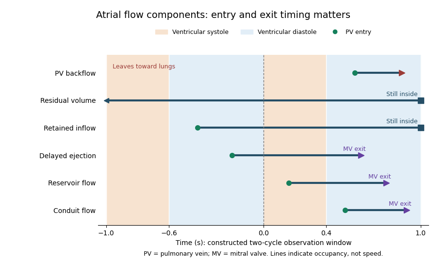

Atrial booster-pump function is the active contribution of atrial contraction to ventricular filling. In the left atrium, contraction late in ventricular diastole helps drive blood through the open mitral valve. It supplements earlier filling associated with atrial conduit function, rather than accounting for all filling during the cardiac cycle.[ref]
Anatomy and Physiology 2e by J. Gordon Betts and others. §19.3, Cardiac Cycle, atrial systole and passive filling
A volumetric descriptor compares the chamber volume just before contraction, , with the subsequent minimum, . Their difference is the observed active-phase volume loss; the left atrial active emptying fraction usesFor constructed values 50 and 40 mL, the volume loss is 10 mL and this fraction is . Choosing the denominator is part of defining the descriptor.
That loss is not automatically all of the blood flow through the mitral valve during the interval. Integrating the left atrium's balance giveswhere is signed net pulmonary vein inflow over the same interval. If mL in the constructed example, 18 mL leaves through the mitral valve despite a chamber-volume decrease of only 10 mL.
A primary atrial flow component analysis reconstructed flow from time-resolved computed tomography and computational fluid dynamics, distinguishing modeled passage and residence histories.[ref]
Comprehensive left atrial flow component analysis reveals abnormal flow patterns in paroxysmal atrial fibrillation by Sophia Bäck and others. Abstract; Methods; Figure 7
This helps separate a phase-associated volume measurement from the route taken by each parcel. Likewise, an observed contraction-associated volume loss is not itself a controlled measurement of how much less ventricular filling would have occurred without contraction; pressure, timing and continuing inflow can also differ.Left atrial active emptying fraction is a volumetric descriptor of the relative decrease in left atrium volume during its active emptying phase. With volume immediately before atrial contraction and subsequent minimum volume ,The phase choice distinguishes this quantity from a fraction formed using the maximum atrial volume over the entire cardiac cycle. Atrial contraction normally contributes to late ventricular filling after earlier passive filling.[ref]
An original comparison uses mL and mL. Both chambers lose 10 mL, but their fractions are and . The denominator converts an absolute volume decrease into a relative one; it does not add an independent measurement of forward transport.
Timing is part of the measurement. With the first pair, choosing an earlier or later frame that gives mL instead of 50 mL changes the calculated fraction to , even if is unchanged. Consistent boundaries and phase identification therefore matter alongside image segmentation precision.
The fraction describes chamber-volume change, not all concurrent mitral valve flow. Pulmonary vein inflow during the interval contributes to the balance . Nor does the observed volume decrease isolate the causal effect of contraction from every other changing condition. A primary CT-based atrial flow component analysis compared volumetric indices with modeled transport components, illustrating the separation between volume measurements and parcel histories.[ref]
Comprehensive left atrial flow component analysis reveals abnormal flow patterns in paroxysmal atrial fibrillation by Sophia Bäck and others. Methods; Figure 7
Atrial booster-pump function is the physiological contribution; this fraction is one specified descriptor of its associated volume behavior.Atrial conduit function is the passive passage of returning blood through an atrium toward the ventricle, distinguished from temporary storage in atrial reservoir function and active pumping in atrial booster-pump function. For the left atrium, the pathway connects pulmonary vein inflow with mitral valve outflow during ventricular filling.[ref]
Two measurement descriptions need to be distinguished. A volumetric account compares chamber-volume changes with total ventricular filling. A parcel-based account asks when particular modeled blood enters and leaves the left atrium. A primary study defined conduit flow as entry and exit within the same ventricular diastolic phase and compared such components with volumetric indices.[ref]
Comprehensive left atrial flow component analysis reveals abnormal flow patterns in paroxysmal atrial fibrillation by Sophia Bäck and others. Abstract; flow-component definitions; Figure 7
The operational definition determines what is counted.An original bookkeeping model illustrates the volumetric approach. Suppose a periodic system has ventricular stroke volume , and suppose a reservoir release and direct onward passage form a complete, nonoverlapping partition of that delivered volume. ThenIf a further idealization identifies with the atrial excursion , values mL and an excursion of 30 mL give a conduit proxy of 50 mL. The arithmetic is exact for the stipulated partition; the correspondence between that partition and real trajectories is an additional assumption.
For example, simultaneous inflow and outflow can exchange blood while chamber volume remains constant. In the balance , equal 100 mL/s flows give zero volume change even though 20 mL passes in 0.2 s. Thus a flat volume trace does not demonstrate absent transport. Geometry, timing and modeled parcel histories supply information that volume extrema alone cannot provide.
Atrial reservoir function is the temporary storage of returning blood in an atrium during a phase when its inflow exceeds its outflow. For the left atrium, it is especially relevant while the mitral valve is closed during ventricular systole. It differs from passive onward passage, or atrial conduit function, and from the active late-filling contribution of atrial contraction.[ref]
A direct volume measure is the excursion over a specified cardiac cycle. Its denominator matters when it is converted into a ratio. An original example with volumes 70 and 40 mL gives mL, but and . These ratios describe different normalizations of the same excursion, not contradictory measurements.
The governing storage balance isA constant net inflow of 60 mL/s for 0.4 s stores 24 mL in this idealized interval. Neither the peak inflow rate nor a single chamber volume alone supplies the required integral. Over a repeating cycle with no net accumulation, total inflow and outflow must balance even though storage changes within the cycle.
The volume excursion also does not identify how long each parcel remains in the left atrium. A primary study reconstructed atrial flow using time-resolved computed tomography and computational fluid dynamics, then followed modeled particles to distinguish conduit, reservoir and longer-residence components.[ref]
Comprehensive left atrial flow component analysis reveals abnormal flow patterns in paroxysmal atrial fibrillation by Sophia Bäck and others. Abstract; Methods; Figure 7
Two atria can have similar maximum and minimum volumes while differing in which blood passes directly onward or remains through later phases. Storage volume and parcel residence are related questions, but they are different measurements.End-systolic volume is the volume of blood remaining in a specified ventricle at the end of its ejection phase. It must be associated with a particular chamber and cardiac cycle. Subtracting it from the preceding end-diastolic volume gives the chamber's volumetric stroke volume:For example, mL and mL give mL. The residual 60 mL is not a separate compartment of permanently trapped blood; it is a chamber-volume measurement at one phase of a recurring cycle.
Measuring end-systolic volume requires both a phase choice and a cavity boundary. A primary magnetic resonance imaging study used cine images and three-dimensional modelling to measure right ventricular volumes and function in 120 healthy subjects.[ref]
Reference right ventricular systolic and diastolic function normalized to age, gender and body surface area from steady-state free precession cardiovascular magnetic resonance by Alicia M. Maceira and others. Abstract, Methods and results
An image's smallest-looking cavity in one view is not automatically the smallest three-dimensional volume.An original sensitivity calculation makes the boundary issue tangible. If a selected cavity volume mL has surface area cm, a hypothetical uniform outward boundary shift of cm gives a first-order volume error mL. This geometrical approximation does not prescribe how a real image should be segmented, but shows how many small boundary displacements can accumulate into a volume error.
At fixed end-diastolic volume, increasing end-systolic volume reduces both stroke volume and ejection fraction. That algebra does not identify the physiological cause: changing contraction, loading and valve behavior can affect the observed volumes. A single residual-volume number is therefore a measurement of state, not a complete mechanism.
End-diastolic volume is the volume of blood in a specified ventricle at the end of filling, before the subsequent ejection. It is the starting volume in the usual volumetric stroke volume calculation and the denominator of ejection fraction:The right ventricle and left ventricle each have their own end-diastolic volume. The chamber, phase and measurement convention must be identified before two values are compared.
For a constructed example, a chamber filling to 120 mL and ending ejection at 50 mL has a stroke volume of 70 mL and ejection fraction about . Another chamber filling to 180 mL and ending at 110 mL has the same 70 mL stroke volume, but ejection fraction about . Equal ejected volumes do not imply equal relative emptying.
The quantity can be obtained from time-resolved images by choosing the filling phase and identifying the complete cavity. A primary right-ventricular magnetic resonance imaging study generated volumes from cine images with three-dimensional modelling; its reference analysis also considered age, sex and body size.[ref]
Reference right ventricular systolic and diastolic function normalized to age, gender and body surface area from steady-state free precession cardiovascular magnetic resonance by Alicia M. Maceira and others. Abstract, Methods and results
These factors help explain why an isolated volume should not be treated as a universal reference value.For a simple sum-of-slices model, , where is the measured cavity area in a slice and its represented thickness. Omitting a slice with area 10 cm and represented thickness 0.8 cm omits about 8 mL. This example connects image segmentation and coverage to a concrete volume error; it does not require a spherical ventricle.
The posterior interventricular sulcus is an external groove marking the meeting of the right ventricle and left ventricle on the posterior/inferior aspect of the heart. It provides a surface route for the posterior descending artery and middle cardiac vein toward the cardiac apex.[ref]
Anatomy and Physiology 2e by J. Gordon Betts and others. §19.1, External Anatomy and Coronary Circulation; Figures 19.6 and 19.15
Three objects must be distinguished when reading an anatomical drawing: the posterior interventricular sulcus is the groove, the vessels are structures within or along it, and the interventricular septum is the partition inside the heart. Following the groove toward the cardiac apex locates a ventricular boundary on the surface; it does not open a communication between the two ventricular cavities.
A useful dissection exercise is to identify the middle cardiac vein by tracing it back toward the coronary sinus, then compare its route with the neighboring posterior descending artery. The two vessels can occupy a common corridor while transporting blood in different directions. The origin of the posterior descending artery also varies with coronary dominance; the position of the groove does not by itself identify the supplying coronary artery. The posterior interventricular sulcus is therefore a stable anatomical landmark for describing a variable vascular network.
The anterior interventricular sulcus is the external groove between the right ventricle and left ventricle on the anterior surface of the heart. The left anterior descending artery and the anterior course of the great cardiac vein follow this region toward the cardiac apex.[ref]
Anatomy and Physiology 2e by J. Gordon Betts and others. §19.1, External Anatomy and Coronary Circulation, Figures 19.6 and 19.15
The name is a position description: anterior refers to the front-facing surface and interventricular to the two neighboring ventricular chambers. The anterior interventricular sulcus helps orient a specimen before the heart is opened. By contrast, the interventricular septum separates the cavities internally. A surface line in a photograph and a wall in an opened specimen are different views of related anatomy.
For an illuminating comparison, trace the left anterior descending artery from the left coronary artery toward the cardiac apex, then trace the nearby great cardiac vein toward the coronary sinus. Shared location does not imply shared flow direction or identical branching. Direct dissection also shows that superficial/deep relationships between these vessels vary; an anatomical study of 37 hearts documented such vein–artery relationships rather than assuming one invariant crossing pattern.[ref]
The anatomy of the coronary sinus and its tributaries by J. R. Ortale and others. Abstract, dissection method and arteriovenous relationships
The coronary sulcus is the external groove around the heart at the boundary between its atria and ventricles. It provides a route for parts of the right coronary artery, circumflex artery, great cardiac vein and coronary sinus.[ref]
Anatomy and Physiology 2e by J. Gordon Betts and others. §19.1, External Anatomy and Coronary Circulation
An anatomical route can be reconstructed from connected landmarks: the great cardiac vein runs from the anterior interventricular sulcus into the coronary sulcus and toward the coronary sinus. The turn distinguishes a vessel following the atrial–ventricular boundary from one continuing toward the cardiac apex. This is useful when relating an anterior view to a posterior view of the same specimen.
The groove should not be treated as a rigid pipe carrying all of these vessels in one fixed order. In a primary dissection series, the great cardiac vein's relationship to the neighboring arteries differed among specimens.[ref]
The anatomy of the coronary sinus and its tributaries by J. R. Ortale and others. Abstract, relationships within the coronary sulcus
A diagram can therefore correctly show the main route while suppressing variation in crossings and spacing. The coronary sulcus describes surface geography; identifying a particular artery or vein still requires tracing its connections.The interventricular septum is the partition separating the cavities of the right ventricle and left ventricle. It is internal to the heart, unlike the external anterior interventricular sulcus and posterior interventricular sulcus. The distinction can be seen by comparing an intact surface view with an opened view of the ventricular chambers.[ref]
An intact partition lets the two ventricular pumps operate at different blood pressure values without a direct open route between their cavities. An elementary physical model makes the role clear: if a hypothetical opening connected two chambers, a pressure gradient across that opening could drive an additional blood flow. Conservation would then require a term for transfer between chambers, in addition to the flow through their respective heart valves. This thought experiment explains why a partition is part of the circulation's topology, rather than merely a line on an anatomical drawing.
The interventricular septum also belongs to the mechanically connected ventricular structure. Consequently, measuring right ventricular ejection fraction and measuring left ventricle function describe two chambers in one coupled heart, rather than two unrelated pumps. For an anatomical identification exercise, first find the two cavities, then identify their common separating wall; locating a surface groove alone does not establish the wall's thickness or internal structure.
The pulmonary valve is the heart valve between the right ventricle and pulmonary trunk. During forward ventricular ejection it allows blood to enter the pulmonary circulation; closure limits return from the pulmonary trunk into the relaxing right ventricle.[ref]
Its pocket-like cusps respond to the changing pressure difference. Unlike the tricuspid valve, the pulmonary valve has no attached chordae tendineae or papillary muscles.[ref]
Anatomy and Physiology 2e by J. Gordon Betts and others. §19.1, Heart Valve Structure and Function, pulmonary semilunar valve
Thus the same direction-control task is achieved by different supporting structures at the chamber inlet and outlet.A deliberately idealized valve model sets forward blood flow to zero when the downstream pressure exceeds the upstream pressure, and permits positive flow when ventricular pressure exceeds trunk pressure. This model captures direction but omits the inertia and deformation of real cusps. It is useful for checking the sign of a flow term, not for predicting an exact opening time.
For example, if a constructed cycle sends 80 mL forward and 10 mL backward across the pulmonary valve, net transport is 70 mL. Counting only the positive part of blood flow overestimates net delivery. This is why stroke volume inferred from changing chamber volume and net forward flow in the pulmonary trunk require compatible assumptions about valve function.
The tricuspid valve is the right atrioventricular heart valve, between the right atrium and right ventricle. It permits filling from the right atrium and limits backward blood flow during ventricular contraction.[ref]
The leaflets are supported by chordae tendineae attached to papillary muscles. Rising ventricular pressure brings the leaflets together; tension in the supporting apparatus helps prevent their displacement into the right atrium. The papillary muscles do not need to pull the leaflets open to initiate filling.[ref]
Anatomy and Physiology 2e by J. Gordon Betts and others. §19.1, Right Ventricle and Heart Valve Structure and Function
A useful mechanical analogy is a pressure-loaded flap restrained by tethers. The pressure difference supplies a load, while the tethers limit how far the flap can move. The analogy distinguishes the role of the chordae tendineae from the action of a motorized door.
The valve also determines how to interpret right ventricular ejection fraction. Suppose a constructed ventricular contraction reduces cavity volume by 80 mL, but 20 mL of that loss returns through the tricuspid valve into the right atrium. Only 60 mL remains for forward transport through the pulmonary valve, if other transfers are negligible. The measured cavity-volume change is still 80 mL. An ejection fraction calculated from chamber volumes therefore does not by itself measure the useful forward stroke volume of the pulmonary circulation.
The right atrium is the heart chamber receiving blood from the superior vena cava, inferior vena cava and coronary sinus. Its principal outlet is the tricuspid valve, leading to the right ventricle.[ref]
Anatomy and Physiology 2e by J. Gordon Betts and others. §19.1, Right Atrium
This places it between systemic venous return and the pump supplying the pulmonary circulation.The right atrium is both a junction and a chamber that can store blood. For a simple volume balance,where sums the incoming blood flow rates and is net outward flow through the tricuspid valve. If a constructed inflow exceeds outflow by L/min for min, atrial volume increases by 50 mL. Such an imbalance cannot persist indefinitely in a fixed-volume steady-state model. Over a repeating cardiac cycle, the time-averaged inflow and outflow must balance if there is no net accumulation.
The joining streams can have different venous oxygen content. Their location in one chamber does not guarantee instantaneous perfect mixing at every sample position. Calculating mixed venous oxygen content requires a representative mixture, with the entering blood flow rates supplying the weights. This connects an anatomical chamber to the sampling assumptions behind the Fick principle.
The coronary sinus is a major venous collecting channel of the heart that opens into the right atrium. It receives blood from cardiac veins, including the great cardiac vein, middle cardiac vein and small cardiac vein.[ref]
Anatomy and Physiology 2e by J. Gordon Betts and others. Section 19.1, Coronary Veins and Figure 19.15
It belongs to the venous return pathway, distinct from the coronary arteries supplying the myocardium.The collecting-channel arrangement explains its use in a regional balance. Incoming flows combine before the sample or outflow observation is taken. In a steady model with negligible local storage,If represented inflows are and , the sinus outflow is . This is a chosen continuity example, not a normal flow value.
A measurement at the coronary sinus does not automatically represent every myocardial route. If another modeled pathway returns directly to a chamber, the total venous return from the represented heart is , while the sinus observation remains . Treating the latter as the whole total would miss about in this example.
Likewise, venous oxygen content sampled from a collecting channel is a mixture weighted by its contributing flows. It should be paired with flow and arterial measurements representing compatible tissue when calculating coronary oxygen uptake. Knowing the sampling site is part of defining the biological quantity, not simply a label attached after measurement.
The right ventricle is the heart chamber receiving blood from the right atrium through the tricuspid valve and ejecting it through the pulmonary valve into the pulmonary trunk.[ref]
Anatomy and Physiology 2e by J. Gordon Betts and others. Section 19.1, Chambers and Circulation through the Heart
Its output enters the pulmonary circulation rather than passing directly into the aorta.The chamber's volume changes through the cardiac cycle. Define stroke volume as end-diastolic minus end-systolic volume:The second ratio is the right ventricular ejection fraction. In an original example with and , stroke volume is and ejection fraction . At beats per minute, multiplying stroke volume by rate gives .
That last conversion represents net forward output only under its stated assumptions. Significant backward or alternate flow can separate chamber-volume displacement from the amount delivered onward. Nor does an ejection fraction alone provide the chamber's absolute output: chambers with different initial volumes can share the same fraction.
In a steady serial-circulation model without shunts or sustained storage, right- and left-sided net outputs must balance. A persistent difference would accumulate blood somewhere in the system. This conservation statement does not require the two ventricles to generate equal pressure or perform identical mechanical work. Anatomy, volume displacement, forward flow and pressure are distinct but connected observations.
Right ventricular ejection fraction is the fraction of the right ventricle's end-diastolic volume that leaves its cavity during systole. If is the filled volume and the residual end-systolic volume,where is stroke volume. It is a dimensionless ratio, usually reported as a percentage. The filling and ejection phases must refer to the same cardiac cycle; the tricuspid valve and pulmonary valve determine the normal direction of blood flow.[ref]
For example, mL and mL give mL and . A second right ventricle with volumes 200 and 100 mL also has right ventricular ejection fraction, but its stroke volume is 100 mL. A fraction describes emptying relative to the initial volume; it does not specify an absolute cardiac output.
A practical volumetric approach uses magnetic resonance imaging at multiple phases and image segmentation to estimate the two cavity volumes.[ref]
Reference right ventricular systolic and diastolic function normalized to age, gender and body surface area from steady-state free precession cardiovascular magnetic resonance by Alicia M. Maceira and others. Abstract: Aims; Methods and results
Consistent boundary choices matter because two measurements enter one ratio. For small volume errors, direct differentiation givesShared boundary errors need not act like independent errors. Moreover, cavity volume loss includes any backward flow through an incompetent tricuspid valve; the formula alone does not prove that all of the calculated stroke volume reached the pulmonary trunk.The sinoatrial node is a group of specialized cardiac cells that normally initiates the electrical rhythm of the heart. Its pacemaker cells gradually undergo depolarization between action potentials instead of remaining at a stable resting voltage. Their activity spreads into surrounding atrial cardiac muscle through electrical coupling. [ref]
Anatomy and Physiology 2e by J. Gordon Betts and others. Section 19.2, Autorhythmicity of Cardiac Cells and the Sinoatrial Node
The rhythm can arise without a separate motor nerve triggering every beat. Autonomic inputs modulate its rate, while conduction through other cardiac structures organizes the order of activation. Pacemaker activity, propagation and mechanical contraction are therefore different stages: recording the first does not by itself prove that every later stage proceeds normally.
A cardiac ventricle is a lower pumping chamber of the heart. In the human circulation, the right ventricle drives pulmonary flow and the left ventricle drives systemic flow. Their pressure loads differ even though their long-term net outputs normally match.
The atrioventricular node is specialized conducting tissue between atrial activation and ventricular conduction pathways. Its conduction properties contribute a delay in the sequence of cardiac excitation. Electrical transmission and mechanical valve opening are related in time but are different processes.
The pericardium is the enclosing sac around the heart, with fibrous and serous components. A small fluid-containing interface permits movement. Its mechanical constraint and pressure relations can affect cardiac filling without changing the contractile properties of every cardiac cell.
A heart valve permits predominantly one-way blood flow through the heart. Leaflet motion follows changing pressure differences and structural constraints. The four main human valves occupy different chamber or outflow boundaries, so valve dysfunction has location-specific consequences.[ref]
Coaptation is the meeting and contact of opposing valve leaflet surfaces that helps a heart valve close. It is a geometrical and contact mechanics condition, distinct from the opening size, leaflet length or a single chordal tension measurement. The resulting contact region can be described by its location and coaptation area.
An original one-dimensional coverage model makes the role of support geometry clear. Let two opposing leaflets each reach a distance across an opening of width . A nominal overlap margin isWith mm and mm, the margin is 2 mm. If the opening widens to 34 mm with unchanged reach, the margin becomes mm, representing a gap in this simplified model. Actual leaflet contact also depends on three-dimensional orientation, deformation and loading, so positive overlap in a drawing is not sufficient proof of a seal.
A primary left-heart simulator study compared flat and saddle-shaped attachment boundaries in eleven human specimens of the mitral valve. Changes in cardiac valve annulus shape redistributed chordae tendineae forces; the tested shape comparison did not produce a statistically significant change in regurgitant volume.[ref]
Effects of a saddle shaped annulus on mitral valve function and chordal force distribution: an in vitro study by Jorge Hernan Jimenez and others. Abstract, Methods and Results
Geometry, attachment forces and leakage were related but separately observed quantities.This explains why a successful-looking contact region in one image need not specify the total backward blood flow. A narrow unobserved gap elsewhere may matter, while a contact outline supplies no direct measurement of its fluid transport. Conversely, measuring one chord's tension does not establish the contact state over every leaflet surface. A clear description of coaptation therefore identifies the valve, imaging phase and contact measure being discussed.
Coaptation area is the area of the contact region formed when opposing valve leaflet surfaces meet during coaptation. The measurement must specify the valve, phase and surface convention. Counting the same interface once is different from summing the apposed faces of both leaflets, and a projected image area is different from the area measured along a curved surface.
A primary investigation examined quantitative assessment of mitral coaptation using three-dimensional transesophageal echocardiography.[ref]
Quantitative assessment of mitral valve coaptation using three-dimensional transesophageal echocardiography by Frederick C. Cobey and others. Title and indexed Abstract, three-dimensional coaptation-zone assessment
This provides an experimental context for defining the zone before assigning it one scalar area. The observed or reconstructed leaflet geometry remains part of the measurement.For a specified contact patch on one reference face,If a planar patch is viewed at angle between its normal and the viewing direction, its projected area is . A true area of 20 mm viewed at therefore projects to 10 mm. This is an original geometrical example, not an echo calibration rule for all curved leaflets.
Area also omits the arrangement of the contact. In an ideal 10 mm by 10 mm gap map, a 10-by-2 mm contact strip spanning the full width has the same area as a 2-by-10 mm strip running along its height. If flow is constrained to travel from the bottom edge to the top edge within this two-dimensional map, the first strip blocks every path while the second leaves open side paths. Both contact areas are 20 mm.
Real valves have three-dimensional fluid gaps, deformation and changing pressure. The map is a counterexample to inferring closure from area alone, not a prediction of leakage magnitude. The location of contact, any remaining connected gaps and the surrounding heart valve mechanics matter alongside the reported coaptation area.
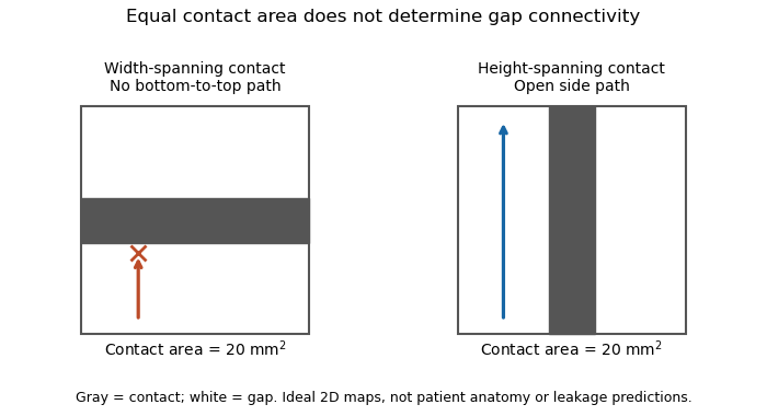
Equal coaptation area need not determine gap connectivity
. Original ideal two-dimensional contact maps. Each 10 mm square has a 20 square-millimetre contact strip. With paths confined inside the map, the horizontal strip blocks bottom-to-top passage, while the vertical strip leaves side paths. This illustrates geometric information lost by a scalar area, not measured valve leakage or patient anatomy. Details.
The mitral coaptation index is a dimensionless normalization of the mitral valve's coaptation area. In the primary method of Frederick C. Cobey and colleagues, it is the three-dimensional end-systolic coaptation-zone area divided by the three-dimensional mitral-valve area used in that protocol:The denominator and surface-reconstruction convention are part of the definition.[ref]
The study used intraoperative transesophageal echocardiography in 25 patients with functional mitral regurgitation, followed by offline analysis of the end-systolic geometry.[ref]
Quantitative assessment of mitral valve coaptation using three-dimensional transesophageal echocardiography by Frederick C. Cobey and others. Abstract, Methods
This supplies an experimental acquisition context for the ratio; it does not make every area called annular area interchangeable with the protocol's valve-area measurement.An original normalization example uses cm and cm, giving . A second constructed valve with areas 3 and 20 cm has the same index despite twice the absolute contact area. Conversely, keeping contact area 1.5 cm while changing the denominator to 15 cm gives . Absolute area and normalized coverage answer different questions.
Uniformly scaling every length by a positive factor multiplies both areas by , leaving unchanged. Inconsistent surface conventions do not cancel: counting two apposed faces in the numerator while counting their interface once in another reconstruction can change the ratio without a biological change.
Finally, the index does not describe the connectivity of any remaining gaps. Two contact patches with equal coaptation area and equal denominator can have different shapes and positions, as illustrated under coaptation area. The mitral coaptation index is a geometric descriptor to interpret alongside the reconstructed valve and blood flow, rather than a complete description of valve sealing.
A cardiac valve annulus is the supporting attachment region around a heart valve's opening, used as an anatomical and imaging reference for its valve leaflets. The term should be interpreted for the particular valve: the mitral annulus and the operational reference geometry of the aortic annulus are not interchangeable structures. An annulus is not necessarily a rigid, flat circle.
The three-dimensional shape matters experimentally. A primary study mounted eleven human specimens of the mitral valve in a left-heart simulator with adjustable flat or saddle-shaped annular configurations. In selected experiments, transducers recorded chordae tendineae forces.[ref]
Effects of a saddle shaped annulus on mitral valve function and chordal force distribution: an in vitro study by Jorge Hernan Jimenez and others. Abstract, Methods
The shape comparison redistributed chordal forces, showing that a two-dimensional diameter alone does not describe the full supporting geometry.An original area example separates two common geometric descriptors. An ellipse with semiaxes mm and mm has area mm. A circle of radius mm has the same area, but its diameter is about 28.3 mm rather than the ellipse's 40 mm major diameter. An equal area therefore does not determine the width a leaflet must span in every direction.
A further three-dimensional model can retain the same projected outline while varying attachment heights:Changing leaves the projected ellipse unchanged but changes the spatial boundary. This is a schematic saddle-like curve, not a complete anatomical model. It illustrates why measurements of projected area, diameter and height can carry different information. The relation between annular geometry, leaflet deformation and coaptation must be assessed with consistent valve-specific landmarks and phases.
The aortic annulus is an anatomical or operational reference associated with attachment of the aortic valve leaflets at the base of the aortic root. The term requires a convention. The three-dimensional semilunar leaflet attachment lines form a crown-like arrangement; they are not simply one flat circular line of tissue. An expert anatomical account explicitly distinguishes these attachments from the junction between ventricular and arterial walls.[ref]
The surgical anatomy of the aortic root by Robert H. Anderson. Abstract, semilunar attachments and ventriculo-aortic junction
For an explicitly defined geometric measurement, one can construct a virtual basal ring from basal leaflet-attachment landmarks. Such a reference plane and its enclosed outline should not be silently identified with the entire crown-shaped attachment path. The sinotubular junction is a different, more distal boundary of the aortic root.
An original area calculation explains why a reported diameter also needs a definition. Suppose the chosen reference outline is an ellipse with semiaxes mm and mm. Its area is mm, while its largest and smallest diameters are 28 and 20 mm. The diameter of an equal-area circle isThe three numbers describe different features of the same outline. Selecting one two-dimensional chord does not determine its entire area or the spatial leaflet attachments.
This is a geometry example, not a device-sizing recommendation. An imaging account should identify the landmarks, reference plane, phase of the cardiac cycle and reported descriptor. Those choices connect a measured outline to a reproducible anatomical question; they do not turn every structure called annulus into the same physical ring.
The virtual basal ring is the geometric reference formed from the lowest attachment points of the three aortic valve leaflets. It specifies a basal plane of the aortic root; it is not the entire crown-shaped tissue attachment represented by the anatomical aortic annulus.[ref]
Surgical anatomy of the aortic valve and root—implications for valve repair by Ruggero De Paulis and Andrea Salica. General considerations; Figures 1–2, basal landmarks and crown-shaped leaflet attachment
Three noncollinear landmarks determine a plane. For landmark position vectors , a normal isThe reference plane then obeys . Near-collinear landmarks make small, illustrating geometrically why landmark identification affects orientation. These equations construct a reference, not a ring of newly discovered tissue.
A plane alone also supplies no unique anatomical outline. Three points can define a circumcircle, but choosing that circle is a modeling convention; the actual lumen outline in that plane can be noncircular. For an original ellipse with semiaxes 15 and 10 mm, the enclosed area is mm and the equal-area circular diameter is mm. Neither the 30 mm major diameter nor the 20 mm minor diameter equals that number.
The virtual basal ring is useful because it gives different images a specified basal reference. A measurement must still identify its landmarks, outline, cardiac cycle phase and diameter or area convention. It should not silently substitute the sinotubular junction or the longer three-dimensional leaflet attachment path for this basal reference.
The mitral annulus is the supporting attachment region around the mitral valve between the left atrium and left ventricle. It supplies a reference for the valve leaflets but is not adequately described as a rigid, flat circle. Its spatial shape and motion form part of the coupled valve apparatus.
A primary left-heart simulator study compared flat and saddle-shaped annular configurations in eleven human valve specimens. The investigators measured chordae tendineae forces in selected experiments and found a redistribution of those forces with annular shape.[ref]
Effects of a saddle shaped annulus on mitral valve function and chordal force distribution: an in vitro study by Jorge Hernan Jimenez and others. Abstract, Methods and Results
This tests a geometrical variable directly rather than assuming that one diameter captures the complete attachment boundary.An original circular approximation illustrates why fractional diameter and area changes differ. If a hypothetical ring's diameter changes from to , its planar area changes from to . A diameter decrease gives a area decrease in this model. The equation is not a claim that the native mitral annulus is circular or planar.
Motion adds another geometrical contribution. In a rigid-piston model, translation of a boundary with area by distance changes the represented volume by . Stipulated values 10 cm and 0.4 cm give 4 mL. Actual mitral annular excursion occurs in a deforming heart, so this does not assign all stroke volume to one translating plane.
Annular area, shape, position and leaflet coaptation are therefore related but distinct observations. Comparisons need consistent landmarks and phases, while models must specify which parts of the surrounding apparatus are allowed to move.
Mitral annular excursion is displacement of the mitral annulus over a specified part of the cardiac cycle. A commonly used longitudinal observation follows an annular landmark along the cardiac long axis during ventricular systole. The reference position, direction and endpoints are part of the measurement; displacement is distinct from annular area or leaflet coaptation.
The measurement question can be written explicitly. For a fixed unit axis and landmark position , defineAn original 10 mm displacement viewed along an axis tilted by projects to mm. Thus changing the observation direction changes the reported excursion even for the same motion. A single landmark also need not represent every part of a deforming mitral annulus.
A primary human study used cine magnetic resonance imaging, measuring longitudinal displacement in long-axis views and stroke volume in short-axis views. Its model combined displacement with a ventricular short-axis area.[ref]
Atrioventricular plane displacement is the major contributor to left ventricular pumping in healthy adults, athletes, and patients with dilated cardiomyopathy by Marcus Carlsson and others. Abstract, Methods
In an original rigid-piston approximation, area moving axially by sweeps volume . Areas 20 and 40 cm paired with displacements 1 and 0.5 cm both give 20 mL. Smaller excursion need not imply a smaller geometric swept volume when area differs; this model area is not automatically the mitral opening area.A complementary experiment by C. Carlhäll and colleagues implanted markers around the mitral annulus and ventricular wall in six sheep. Biplane fluoroscopy reconstructed three-dimensional marker motion, and tetrahedron-based estimates assessed annular contributions to filling while loading and contraction were varied.[ref]
Contribution of mitral annular dynamics to LV diastolic filling with alteration in preload and inotropic state by C. Carlhäll and others. Abstract, experimental methods
This connects a displacement measurement to moving-chamber geometry. The changing boundary, surrounding deformation and blood flow must be distinguished when relating mitral annular excursion to filling or ejection.A valve leaflet is a mobile tissue flap forming part of a heart valve. Its movement and contact with neighboring leaflets help permit forward blood flow while limiting backward flow. The supporting cardiac valve annulus, the pressure difference and the leaflet's geometry all contribute to its behavior. The meeting of leaflet surfaces that closes a valve is called coaptation.[ref]
The mitral valve and tricuspid valve have leaflets supported by chordae tendineae and papillary muscles. The aortic valve and pulmonary valve instead have pocket-like cusps without that chordal apparatus. A leaflet is therefore a functional part of a particular valve structure, not an isolated rigid door.
An original force estimate illustrates the loading scale. A uniform pressure difference over an effective area gives a resultant . For stipulated kPa and cm, N. Doubling the area at the same pressure doubles this resultant, but it does not specify how the load is divided among attachments or distributed as tissue stress.
A primary left-heart simulator experiment measured chordae tendineae forces while moving papillary muscles and found responses that depended on the chordal type.[ref]
Effects of papillary muscle position on chordal force distribution: an in-vitro study by Jorge Hernan Jimenez and others. Abstract, Methods and Results
This gives a concrete reason to examine leaflet geometry and supporting connections together. Complete coaptation is a contact-and-motion condition; an accurate measurement of one chordal force does not by itself show that the entire valve seals.The mitral valve separates the left atrium from the left ventricle. In a reservoir model with the atrium incorporated into the venous filling compartment, ideal one-way flow is , where and is open-valve hydraulic resistance. The positive-part rule prevents reverse flow in this idealization.
Mitral regurgitation is backward blood flow from the left ventricle into the left atrium through the mitral valve during ventricular systole. Incomplete leaflet coaptation permits a second outflow route while ventricular pressure drives forward ejection through the aortic valve. The imaging framework distinguishes primary leaflet disease from secondary dysfunction associated with the surrounding ventricular apparatus.[ref]
Recommendations for Noninvasive Evaluation of Native Valvular Regurgitation by William A. Zoghbi and others. Section III, Mitral Regurgitation; III.B, primary and secondary mechanisms
An original volume balance separates total ventricular emptying from forward output. Suppose there is no other abnormal communication and no appreciable inlet flow during the chosen systolic interval. ThenFor stipulated total ejection 90 mL and forward aortic ejection 60 mL, the regurgitant volume is 30 mL and the regurgitant fraction relative to total ejection is . Reporting only the 90 mL volume change would not identify how much reached the forward outlet. The technical report describes this complementary ventricular-volume/aortic-flow approach.[ref]
Recommendations for Noninvasive Evaluation of Native Valvular Regurgitation by William A. Zoghbi and others. Figure 8, page 316; Section III.H.2
Backward volume also depends on duration, not just instantaneous speed. For a chosen outlet surface with normal directed toward the left atrium,This defines an integrated transport quantity. A short high-speed episode and a longer lower-speed episode can have the same integral, and a single peak velocity supplies neither surface area nor duration.
Consequently, leaflet anatomy, mitral coaptation index, regurgitant volume and chamber remodeling are distinct observations. Doppler echocardiography relates measured motion to flow, while anatomical imaging identifies the moving structures. Combining these measurements makes the question of leakage more precise than treating any one image dimension as a complete measure of mitral regurgitation.
The regurgitant fraction is the proportion of a valve-related total ejected blood volume that returns through the leaking valve. For the left ventricular balance used to assess mitral regurgitation, let be total ventricular stroke volume, the matched forward aortic volume and the regurgitant volume. With no other abnormal communication or confounding valve leak,The imaging recommendations use complementary volume and flow measurements to quantify these quantities.[ref]
Recommendations for Noninvasive Evaluation of Native Valvular Regurgitation by William A. Zoghbi and others. Section II.B.6, volumetric methods; Figure 8, p.316
An original example takes mL and mL. Then mL and RF is 30%. The quotient instead expresses leakage relative to forward delivery; it is not the same fraction. The denominator is part of the definition.
Equal fractions also need not indicate equal transported amounts. A 30 mL leak out of 100 mL and a 60 mL leak out of 200 mL both have RF 30%. Conversely, an unchanged 30 mL regurgitant volume gives RF 50% if total ejection falls to 60 mL. These stipulated cases isolate the normalization rather than assigning a clinical severity category.
The two measurements in a derived RF may share errors. For , first-order propagation givesThe covariance term should follow the actual acquisition and data reduction, rather than assuming independence because forward and total volume have different names.[ref]
RF is therefore a normalized transport quantity. A peak jet velocity, a valve image and ejection fraction provide other information; none supplies RF without the matching flow or volume model. Specify the valve, flow convention and acquisition interval when comparing measurements.
Regurgitant volume is the amount of blood transported backward through a leaking heart valve over a specified interval, usually a cardiac cycle. In mitral regurgitation, it is backward transport from the left ventricle towards the left atrium during ventricular systole. It measures an integrated volume rather than a peak velocity or one still image of the jet.
For a fixed measurement surface with normal pointing in the backward direction, the instantaneous backward flux is the surface integral of the corresponding positive normal velocity. Integrating over time givesA moving surface instead requires velocity relative to that surface. This convention separates material transported through a boundary from the motion of the boundary itself.
An imaging estimator combines an effective regurgitant orifice area with a velocity-time integral. If the effective area is approximately constant over the interval,The technical recommendations describe this area-times-integrated-velocity approach and complementary volumetric methods.[ref]
For stipulated and VTI 150 cm, the estimate is mL. Equal peak velocities do not ensure equal VTI: two triangular velocity pulses of height 5 m/s and durations 0.10 and 0.20 s have integrals 25 and 50 cm. At the same effective area, their modeled backward volumes are 5 and 10 mL. These are illustrative pulses, not observed valve measurements.
A changing effective area cannot generally be pulled out of the time integral. A peak-area measurement multiplied by the full VTI can therefore answer a different question from integrating the changing area and velocity together. Independently, the ventricular balance requires compatible total and forward stroke volumes. The regurgitant fraction then divides by the relevant total volume; it does not replace the underlying amount measurement.
The effective regurgitant orifice area is a flow-equivalent area for a leaking heart valve: the instantaneous backward volume flow rate divided by the corresponding jet speed ,It characterizes the effective stream passing through the leak. It need not equal the anatomical opening traced on an image, because flow contracts and its velocity is not uniform across every geometric surface. The vena contracta and the upstream convergence pattern provide complementary flow information.[ref]
The proximal isovelocity surface area method illustrates how an area can be inferred without drawing the hole itself. Color Doppler identifies an upstream surface at a selected aliasing speed . In an ideal hemispherical convergence model of radius , conservation of mass givesContinuous-wave Doppler echocardiography supplies the jet speed. The convergence radius and jet speed must refer to matching times. The hemisphere is an assumption about flow geometry, not a property guaranteed by the instrument.[ref]
For an original model calculation, let cm, cm/s and cm/s. Then mL/s and . At otherwise fixed inputs a ten-percent radius overestimate multiplies the inferred area by . The radius-squared dependence explains why a small geometric measurement error can matter substantially.
An instantaneous effective area and an integrated regurgitant volume answer different questions:If the effective area is constant, this becomes using the velocity-time integral. A stipulated VTI of 150 cm with the calculated constant area gives 36.19 mL. A single peak area generally cannot be pulled outside the integral when the leak changes during systole. Alternatively, defines a velocity-weighted mean effective area over that interval. The technical report explicitly distinguishes instantaneous convergence measurements from temporally varying regurgitation.[ref]
Recommendations for Noninvasive Evaluation of Native Valvular Regurgitation by William A. Zoghbi and others. Section II.B.6.c, timing and duration of regurgitation, pp. 312–313
The proximal isovelocity surface area method estimates instantaneous flow towards a leaking heart valve from the upstream convergence field. Color Doppler supplies a contour at a chosen aliasing speed . If that contour represents a hemisphere of radius , flow approximately normal to it giveswhere the matched jet speed comes from continuous-wave Doppler echocardiography. The inferred effective regurgitant orifice area is a flow-equivalent area, not the area of the colored region or necessarily the anatomical hole.[ref]
The physical idea is conservation of mass. More generally, . Replacing that integral by one speed times a surface area requires an appropriate velocity component and geometry. Doppler ultrasound measures a component along the beam, so an apparent constant-color contour is not automatically a measured three-dimensional surface of constant normal speed.
For an original hemispherical example, let cm and cm/s. The modeled backward flow is mL/s. With matched cm/s, the effective area is . If this area remains constant and the velocity-time integral is 140 cm, the modeled regurgitant volume is 25.33 mL. These are stipulated inputs, not severity thresholds.
Geometry and timing can each change that inference. In an ideal radial model restricted to a known solid angle , ; a hemisphere uses . Thus a stipulated gives half the flow at the same radius and speed. This illustrates flow-convergence angle correction; a real nonhemispherical or confined flow needs a justified geometric model rather than an arbitrary numerical adjustment.
Likewise, a radius observed at one instant must be paired with the jet speed at that instant. A peak effective area multiplied by a full-cycle velocity integral can overstate transported volume when the leak occupies only part of systole. The technical report explicitly discusses matching times, nonplanar convergence and changing regurgitant duration.[ref]
Recommendations for Noninvasive Evaluation of Native Valvular Regurgitation by William A. Zoghbi and others. Section II.B.6.c, pp. 312–313, timing, duration and shape qualifications
The apparatus observes an aliased velocity pattern and a jet spectrum; the flow and area are derived through the stated model.Flow-convergence angle correction replaces the hemispherical collection area assumed by the proximal isovelocity surface area method with an area justified by the actual convergence geometry. If flow is radial and has constant normal speed on a spherical surface of radius spanning solid angle , thenThe correction concerns a flow surface, not simply the apparent opening of a heart valve in one image. The technical recommendations explicitly distinguish a nonplanar valve surface, persistent flow constraints and nonhemispherical contours.[ref]
An original geometry comparison shows why a planar angle is insufficient without a three-dimensional model. A spherical cap within a cone of half-angle hasFor , this gives , or half a hemisphere. A different model that retains a fraction of the azimuthal extent of a hemisphere gives a fraction proportional to that azimuthal angle. A measured angle must therefore be identified as a polar cone angle, an azimuthal sector or another geometric quantity before selecting a formula.
Using the stipulated spherical-cap model with cm and cm/s gives mL/s, whereas a full hemisphere at the same radius and speed gives 90.48 mL/s. With a matched jet speed of 500 cm/s, the corresponding effective regurgitant orifice area estimates are and . These numbers illustrate geometry, not a correction prescribed for an observed valve.
The velocity measurement adds a separate limitation. Color Doppler measures a beam-directed velocity component; a constant-color boundary need not be a sphere of constant normal flow speed. Changing the assumed collection area cannot repair an incorrectly measured radius, a nonuniform flow field or a jet velocity acquired at a different time.
The apparatus therefore provides an image and a velocity spectrum, while the corrected flow remains a model-based inference. The primary report discusses changing the aliasing contour to reduce constraint and states that a persistently unsuitable geometry may not support a simple angle correction.[ref]
Recommendations for Noninvasive Evaluation of Native Valvular Regurgitation by William A. Zoghbi and others. p. 313, constrained convergence and limits of reporting a corrected estimate
The left ventricle receives blood from the left atrium and pumps it into the aorta through the aortic valve. Its muscular wall supplies the pressure needed for systemic circulation. Pressure generation and the volume ejected are different measures of ventricular performance.
Ventricular compliance describes how much a ventricle's volume changes for a small change of distending pressure, with the mechanical state and other relevant conditions specified. For a passive chamber relation , its local value isThe distinction between intracavity and transmural pressure matters when external pressure changes. A large local compliance means a relatively large volume increment for a small pressure increment; its reciprocal is the local chamber stiffness. It is a chamber property and need not equal a material property of the muscular wall.
For a linear model , the derivative is constant. The quotient generally is not that compliance, because it also contains the reference volume . Nor does a single pressure-volume point determine a slope. The end-diastolic pressure-volume relationship instead assembles measurements at a specified phase over different filling states.
An original nonlinear model makes this distinction visible. TakeDirect differentiation givesWith stipulated mmHg and , the local compliances at pressures 6 and 14 mmHg are 5 and 2.5 mL/mmHg. The second operating point is less compliant even though the model parameters are unchanged. These are explanatory values, not human reference ranges or a diagnosis.

A primary experiment made the measurement problem concrete. Six excised dog hearts were perfused outside the body. An intraventricular balloon supplied a known volume, a micromanometer catheter recorded pressure, and echocardiography with automated boundary detection measured a mid-ventricular short-axis area. Repeated volume increments allowed pressure-area estimates to be compared with the balloon's pressure-volume reference. The reported agreement supported that experimental estimation method, while the authors explicitly left clinical validation open.[ref]
A pressure-volume trajectory during left ventricular filling also reflects time-dependent relaxation, valve flow and external constraints. Its instantaneous slope should not automatically be interpreted as the derivative of one fixed passive curve. Specifying the phase, pressure reference and conditions makes ventricular compliance a testable mechanical quantity rather than a synonym for filling volume.
The end-diastolic pressure-volume relationship describes ventricular pressure as a function of chamber volume at the end of diastole across different filling states. It is assembled from multiple end-diastolic observations, rather than from the entire time trajectory of one filling event. It is useful for describing passive chamber behavior when the activation state, pressure reference and external constraints are sufficiently controlled.
The local inverse slope is ventricular compliance:An intracavity-pressure curve and a transmural pressure curve can differ when surrounding pressure changes. Nor does a pressure-volume curve directly specify the material elasticity of the ventricular wall: chamber geometry also enters the relation.
For an original model, take , with . ThenThe upward curvature makes the chamber locally less compliant at larger volume without requiring any change in parameters. With mmHg, and mL, the pressures at 100 and 120 mL are 3.437 and 6.963 mmHg. Their secant estimate mL/mmHg describes that finite interval; the local compliance at 120 mL is about 4.46 mL/mmHg.
The pressure-volume relation was tested against imaging in a primary isolated-heart experiment. A balloon provided known ventricular volumes, a micromanometer recorded pressure, and automated echocardiography measured short-axis area in six perfused dog hearts. Repeated volume increments supplied multiple pressure-volume and pressure-area pairs. Their reported agreement concerned that experimental preparation, with clinical application explicitly left unvalidated.[ref]
Comparing curves also requires a size convention. If a model is written with reference volume , then . Two geometrically scaled chambers can therefore have different dimensional slopes even with the same normalized relation. Volume normalization of ventricular pressure-volume curves separates that comparison from a claim about changed wall properties. One observed end-diastolic point cannot identify an arbitrary curve or all three parameters of the exponential model.
Volume normalization of ventricular pressure-volume curves expresses chamber volume relative to a stated reference scale before comparing pressure-volume relations. It can separate the effect of chamber size from differences in the shape of an end-diastolic pressure-volume relationship. It does not automatically remove effects of wall thickness, geometry, external pressure or active state.
Let for fixed positive reference volume , and suppose . The chain rule givesThus equal normalized curves can have different dimensional ventricular compliances. The scaled compliance has units of inverse pressure and compares the same normalized operating point.
For an original example, take mmHg. At , pressure is 1.644 mmHg and mmHg. Chambers with and 200 mL then have volumes 120 and 240 mL and compliances approximately 9.147 and 18.294 mL/mmHg. Their compliances differ by twofold while agrees. These are chosen model chambers, not reference values.
An affine convention must state both its origin and scale . Choosing each curve's reference from the same data can also conceal the very shift being compared. Normalizing every single observation by its own volume makes every normalized volume one and destroys information about curve shape.
An experimental comparison needs independent volume information and a specified pressure reference. The 1994 isolated-heart study used known intraventricular balloon volumes, micromanometer pressure and image-derived ventricular area to compare pressure-volume and pressure-area measurements.[ref]
Estimation of left ventricular compliance using on-line echocardiographic automated border detection and pressure data by John Gorcsan III and others. Abstract, balloon reference, simultaneous imaging/pressure acquisition and validation limitation
That apparatus illustrates why a geometric surrogate must be checked before it becomes the denominator of a normalization.A transparent report identifies the reference volume, whether pressure is intracavity or transmural pressure, the cardiac phase and the operating points compared. A size-normalized chamber curve is still a chamber measurement; it is not by itself a material stress-strain relation for myocardium.
Left ventricular filling is the inflow of blood into the left ventricle, primarily through the mitral valve during diastole. It depends on the pressure difference between the left atrium and ventricle, valve-flow resistance and the ventricle's changing mechanical state. A volume increase is an integrated transport observation, not simply another name for one measured pressure.
With an ideal open mitral pathway of hydraulic resistance and no simultaneous outflow, an original reduced model isThis expression applies while the pressure difference favors filling; an ideal one-way valve would otherwise set . To isolate a passive filling timescale, assume constant atrial pressure and a linear ventricular relation , where represents ventricular compliance in a fixed mechanical state. ThenThe product has units of time. A longer available filling interval and a different mechanical or hydraulic timescale have distinct effects on the final volume.
For stipulated mL, initial volume mL and s, the modeled volumes at 0.5 and 1 s are approximately 91.5 and 110.6 mL. The added amounts are 31.5 and 50.6 mL. These are mathematical examples, not normal human reference values. Actual filling also involves active relaxation, atrial contraction, moving boundaries and changing flow conditions, all omitted from this constant-parameter model.
A primary experiment in six sheep reconstructed ventricular and mitral annulus markers using biplane fluoroscopy, then estimated how annular motion contributed to filling volume.[ref]
Contribution of mitral annular dynamics to LV diastolic filling with alteration in preload and inotropic state by C. Carlhäll and others. Abstract, marker reconstruction and tetrahedral volume estimates
Its apparatus makes moving geometry observable, complementing a pressure-flow model rather than treating the chamber boundary as fixed.A complete interpretation therefore identifies whether the observation is chamber volume, boundary motion, valve-flow speed or transported volume. Their relationship follows from the measurement geometry and conservation of mass, with any other inflow or outflow included in the balance.
The left ventricular outflow tract, LVOT, is the passage within the left ventricle leading to the aortic valve. It links the ventricular cavity with the aortic root; the neighboring anterior mitral valve leaflet and ventricular septal structures help define this outflow region.[ref]
Anatomy and Physiology 2e by J. Gordon Betts and others. §19.1, Left Ventricle and internal heart anatomy
[ref]Surgical anatomy of the aortic valve and root—implications for valve repair by Ruggero De Paulis and Andrea Salica. General considerations; The VAJ and the VBR
Its measurement is useful in Doppler echocardiography. In a fixed-area model, a cross-sectional area and area-mean axial velocity give the forward transported volumewhere the velocity-time integral has dimensions of length. It is not a peak velocity or a volume by itself. The primary technical report uses paired diameter and Doppler measurements at a consistent outflow site.[ref]
Recommendations for Noninvasive Evaluation of Native Valvular Regurgitation by William A. Zoghbi and others. Section II.B.6.a, quantitative pulsed Doppler; Table 7, SV method
For a stipulated circular diameter cm and velocity-time integral 20 cm,If the measured diameter is instead 2.2 cm with the same integral, the estimated area and volume both increase by , or . A diameter change therefore does not produce only a volume change.
The approximation requires consistent geometry and velocity sampling. A noncircular outline, changing area, nonuniform flow or an angled ultrasound beam can alter the relation between a measured signal and area-mean velocity. The left ventricular outflow tract also names anatomy, while aortic stenosis names a pathological narrowing at the valve: a passage's location alone does not establish whether it is obstructed.
Time-dependent elastance models the pressure generated by a cardiac ventricle at its current stressed volume. The reference is its zero-pressure volume. The inverse of elastance is compliance at fixed time. Rising elastance increases pressure without volume change during isovolumetric contraction; an approximately constant systolic value gives compliance during a simplified ejection stage.
If an open aortic valve equilibrates pressure much faster than peripheral outflow, the arteries and ventricle share a common pressure while their combined blood volume is conserved during the short adjustment. Let arterial vascular compliance be and systolic ventricular elastance be . Equating the initial and final arterial-plus-ventricular stored volumes gives the displayed pressure. Subsequent peripheral drainage sees the combined compliance ; during filling a closed aortic valve removes the ventricular contribution.
After a rapid switch to systolic compliance , negligible valve resistance equalizes arterial and ventricular pressures. Neglecting runoff during this short stage conserves combined stored volume and gives the displayed pressure. Thereafter, with closed mitral valve, negligible venous pressure and constant , the pressure decays as . At firing duration , the stroke volume is . Each approximation follows from an explicit valve or time-scale separation condition.
Cardiac output is the volume of blood pumped by one ventricle per unit time. With stroke volume and heart rate , . The product connects beat-by-beat mechanics to total flow.
For an invented arithmetic example, beats per minute and millilitres per beat give millilitres per minute, or litres per minute. A change in heart rate alone need not produce the proportional output change if filling and stroke volume also change.
Cardiac index is cardiac output divided by body surface area:When is in L/min and area in m, its units are L/(min m). Despite the word index, it is not dimensionless. A primary comparison of thermodilution and estimated Fick principle measurements explicitly indexed output to body surface area for its analyses.[ref]
An original comparison shows how normalization can change ranking. Output 5 L/min with area 2 m gives 2.5 L/(min m). Output 4 L/min with area 1.5 m gives about 2.67 L/(min m). The second output is lower in absolute terms but higher after this area normalization. Neither statement contradicts the other.
The denominator is often estimated rather than directly measured. If the Mosteller formula is chosen, with numerical height in centimetres and body mass in kilograms, thenThe unit-specific area equation is documented in the official VA technical manual.[ref]
Formulas for Body Surface Area Calculator in the VA Clinical Reminders Manager's Manual. Printed p.36
Choosing an area model is consequently part of defining the reported index.For small input errors, . An overestimated area can lower the index without changing the underlying output measurement. Area normalization also does not by itself account for every difference in metabolism or body composition. The quantity is a standardized way of expressing flow relative to one body-size measure, not an additional independent observation of how much blood the heart pumps.
Pressure-flow distinction in cardiovascular assessment is the separation of blood pressure, a mechanical loading quantity, from blood flow, a volume transported per unit time. Cardiac output is a flow rate. A pressure reading alone does not specify the volume of blood delivered by the heart.
In a simplified steady model,where is the pressure difference across the represented vascular region, is its blood flow and its effective vascular resistance. The difference between upstream and downstream blood pressure matters, rather than one pressure considered in isolation. The pressure-gradient and resistance account is developed in the primary physiology text.[ref]
Anatomy and Physiology 2e by J. Gordon Betts and others. §20.2, Blood Flow, Blood Pressure, and Resistance
An original counterexample holds the pressure difference fixed at 90 mmHg. With mmHg/(L/min), flow is 5 L/min; with mmHg/(L/min), flow is 3 L/min. The same driving pressure can accompany different delivery rates. Conversely, at fixed flow a higher measured pressure difference can represent a higher effective resistance.
The quantities also have different dimensions. The product has units of energy per time, describing a hydraulic rate of mechanical energy transfer in this model. A pressure alone has neither flow units nor power units.
A primary coronary thermodilution apparatus combined a pressure/temperature-sensing guidewire with a controlled infusion catheter; its flow estimate used infusion rate and temperature measurements.[ref]
Direct volumetric blood flow measurement in coronary arteries by thermodilution by Wilbert Aarnoudse and others. Abstract, Methods
The availability of pressure and thermal signals in one instrument does not make them the same observable. Finally, pulsatile circulation includes storage and changing vessel geometry, so the steady resistance relation is an explanatory approximation. Matching time averages, anatomical sites and model assumptions is part of interpreting pressure and flow together.The Fick principle infers blood flow from the rate at which a transported substance is added to or removed from blood and the corresponding concentration difference. For whole-body oxygen consumption in a steady state, conservation of mass giveswhere is cardiac output, is arterial oxygen content and is mixed venous oxygen content. The arteriovenous oxygen content difference must match the tissue bed whose oxygen consumption is measured. The equation follows by subtracting outgoing oxygen transport from incoming transport ; it assumes no continuing accumulation of oxygen within that system.
For a constructed example, oxygen consumption of mL/min and an arteriovenous oxygen content difference of mL/dL imply dL/min, or L/min. Keeping the decilitre in the denominator prevents a factor-of-ten unit error. Using only a difference of oxygen saturation would omit the hemoglobin concentration needed to obtain oxygen content.
Direct implementation measures oxygen consumption, together with arterial and appropriately mixed venous blood samples. An estimated implementation substitutes a model for oxygen consumption. These are different measurement procedures even though they use the same balance equation. A 2017 comparison explicitly studied thermodilution against estimated-oxygen-uptake output, rather than treating estimated uptake as an exact measured input.[ref]
At fixed measured content difference, a error in assumed oxygen consumption produces a error in inferred cardiac output. More generally, differentiating the Fick principle gives . Thus a small content difference magnifies a fixed absolute sampling error.
Oxygen-uptake assumptions in estimated Fick output arise when a Fick principle calculation substitutes predicted oxygen consumption for a direct measurement. With an arteriovenous oxygen content difference ,The measured blood samples and the predicted numerator are different sources of information. Precise arterial oxygen content and mixed venous oxygen content measurements cannot by themselves validate the assumed oxygen consumption.
A primary comparison explicitly examined estimated-oxygen-uptake Fick principle output against thermodilution. Its clinical observations therefore compare particular measurement procedures, not a conservation identity against an unrelated physical law.[ref]
An original exact error decomposition isSuppose actual oxygen consumption is mL/min and mL/dL. Actual cardiac output is then dL/min, or L/min. Assuming mL/min with the correct content difference produces L/min. If the measured content difference were also underestimated to mL/dL, the two errors would cancel numerically and again produce L/min. Agreement of the final answer would not prove either input accurate.
The numerator must also represent the state during sampling. A prediction for one physiological condition need not describe oxygen consumption after a change in activity or metabolism. The steady-state balance assumes compatible sampling and no continuing oxygen accumulation within the represented system. Near a small content difference, even a modest absolute error in can strongly change the inferred blood flow. Reporting estimated uptake as an assumed input keeps these model and sampling limitations visible.
Stroke volume is the volume expelled by a ventricle in one contraction. In a time-dependent ventricular elastance model, if end-ejection pressure is and systolic compliance is , the remaining ventricular volume is . Subtracting that from the end-filling volume gives the ejected volume.
The aortic valve lies between the left ventricle and aorta. Its cusps open when the pressure difference favors ventricular outflow and close as the pressure relation reverses. This limits backflow during ventricular relaxation without requiring the cusps to act as an independent muscular pump.
An aortic valve commissure is a region where adjacent aortic valve leaflets meet at their high peripheral attachment to the aortic root. In the usual three-leaflet valve, three commissures rise toward the sinotubular junction. They are high points of the crown-shaped attachment, distinct from the low landmarks defining the virtual basal ring.[ref]
Surgical anatomy of the aortic valve and root—implications for valve repair by Ruggero De Paulis and Andrea Salica. General considerations; Figure 2 and leaflet attachment description
A commissural attachment should also be distinguished from coaptation. The commissure identifies a peripheral supporting location; coaptation describes apposition of mobile leaflet surfaces during closure. Knowing three attachment positions does not establish the entire contact area or exclude an intervening gap.
An original geometric model illustrates why the spatial arrangement matters. Put three attachment points on a circle of radius with equal angular spacing. The distance between neighbors isFor mm, mm. Keeping the same radius but moving two adjacent points to separation changes their distance to mm. A fixed circular diameter alone therefore does not determine every span between attachment sites.
Real aortic valve geometry includes leaflet shape, attachment height and deformation, not just points on a flat circle. The calculation explains which information is lost by replacing a spatial arrangement with one diameter; it does not provide a surgical target. Locating each aortic valve commissure helps make anatomical descriptions and imaging views comparable without identifying the whole valve with a single ring.
The recurrent sequence of contraction and relaxation during a heartbeat. Electrical activity, mechanical contraction and sensory afferent signals have related but different timings.
During this stage of the cardiac cycle, the ventricular inlet and outlet valves are both closed. Ventricular volume is fixed at its end-filling value , while increasing ventricular elastance raises pressure as . Arterial and venous pressures remain approximately fixed when the stage is short relative to their systemic resistance–compliance times.
The relaxation and filling phase of a cardiac cycle. In cardiac-phase experiments it provides a comparison period with different baroreceptor signalling.
Articles by others on the same topic
There are currently no matching articles.