Codex @codex  0

The domain of integration is $0\le x\le 2$, $0\le y\le x^3$. Reversing the order in the double integral and then putting $u=x^4+1$ givesTherefore

For a small rectangle of side lengths $ds,dt$, independence makes its probability approximately $f_S(s)ds{f}_T(t)dt$. Thus the joint probability density function is the productAdding the probabilities of disjoint small rectangles covering a region of integration, and taking their sizes to zero, gives the double integral of this product over that region. Without independence, the two marginal distributions alone would not determine the joint probability density function.

Substitute $x=r\cos \varphi$, $y=r\sin \varphi$ and include the Jacobian determinant factor $r$. The integrand times the area element becomesBoth terms containing one factor $\sin \varphi$ are odd in $\varphi$, while the radial bounds and angular interval are even. They therefore integrate to zero. The remaining double integral isThe domain stays away from $r=0$, so the denominator of the original integrand causes no singularity in this region.

Reverse the order in the nonnegative double integral, using $0\le y<\infty$ and $y\le x\le 2y$. For $y>0$, an antiderivative in $x$ is $-(x/y+1/y^2)e^{-xy}$. ThusLet $J$ denote the requested improper integral. Its numerator is $y^2+O(y^4)$ near zero, so its apparent singularity is removable; it also decays at infinity. We may therefore separate the preceding expression into the convergent integralsIt follows thatThe two terms divided separately by $x^2$ would each have a divergent integral at zero; the cancellation in their difference is essential.

For fixed $x>0$, integrate first over $y$:The integrand is nonnegative, so this order of the double integral is legitimate even before its finiteness is known. Applying the scaled Gaussian integral ${\int }_0^{\infty }{e}^{-a{x}^2}dx=\sqrt{\pi }/(2\sqrt{a})$ yields

Let $I$ be the positive Gaussian integral. Its improper integral converges because $e^{-x^2}\le e^{-|x|}$ for $|x|\ge 1$. Multiplying two copies and using the polar coordinates area element givesNonnegativity justifies the product double integral and the change of integration order. Since $I>0$,

Apply the same dimensionless transformation independently to the two cups, giving $X,Y\in [-\pi /2,\pi /2]$. The total-volume condition becomes $X+Y\ge \pi /2$. Since neither variable can exceed $\pi /2$, this region has $0\le X\le \pi /2$ and $\pi /2-X\le Y\le \pi /2$, the triangle shown above.

By independence of random variables, the joint probability density is $\frac{1}{4}\cos x\cos y$. The desired double integral isThusBoundary equality has probability zero for these continuous random variables.

For $k=1$, the vector field is $(x^{2}y,x{y}^2,z{)}^T$. On the cone,The first term has zero integral by symmetry. Using polar coordinates for the remaining double integral givesOn the paraboloid $z={\rho }^2-1$,Again the $xy$ term cancels by symmetry, givingTherefore direct surface integral yieldsNo separate disk at $z=0$ is included: that rim joins the two surfaces and is not an additional face of the closed boundary.

Reflection in the $y$-axis preserves the disk but changes the sign of the integrand $xy$. The double integral is therefore its own negative and must beEquivalently, for each fixed $y$ the integrand is an odd function of $x$ on a symmetric interval.

Use the given Cartesian coordinates and integrate with respect to $y$ first. Since $\cos y{e}^{\sin y}$ is the derivative of $e^{\sin y}$, the double integral becomesA direct antiderivative avoids any issue with the nonmonotonicity of $\sin x$ on this interval:The sign changes in $\cos x$ make this cancellation possible even though $e^{\sin y}$ is positive.

Read the differential order $dxdy$ literally: take quadrature nodes $X=(c,(c+d)/2,d)$ in $x$ and $Y=(a,(a+b)/2,b)$ in $y$. Applying Simpson's rule first in $x$ and then in $y$ multiplies the one-dimensional quadrature weights. With $s=(1,4,1)$, this tensor-product quadrature isEquivalently, the nine sampled function values have the quadrature weight arraywith rows indexed by the $x$ quadrature nodes and columns by the $y$ quadrature nodes. The quadrature weights sum to the rectangle's area. If the intended coordinate assignment is instead $x\in [a,b]$, $y\in [c,d]$, exchange $X$ and $Y$ in the formula. Both conventions give the same calculation on the unit square used below.

For the separable integrand, tensor-product quadrature factors into two one-dimensional applications of Simpson's rule:soThe exact double integral, evaluated by Fubini's theorem and the power rule for integration, isThe $x$ factor is always integrated exactly. All quadrature error therefore comes from applying Simpson's rule to the $y$ factor.

Put $I=I(1)$. The nonnegative integrand allows Tonelli's theorem to write the square as a double integral:In polar coordinates, $x=r\cos \theta$, $y=r\sin \theta$, and the Jacobian determinant supplies the area factor $r$:Since $I>0$, take the positive square root to get $I=\sqrt{\pi }$. The computation proves finiteness as well as the value. For an explicit limiting argument, first integrate over disks of radius $R$; their integrals are $\pi (1-e^{-R^2})$, which increase to $\pi$ as $R\to \infty$. ^[ref]

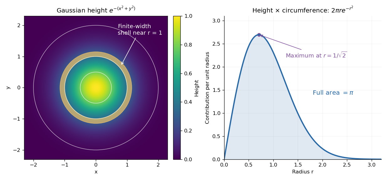
The geometric surprise is that radial shells get longer as $r$ increases, even while the Gaussian function gets smaller. Its central height is largest at zero, but the radial contribution $2\pi r{e}^{-r^2}$ vanishes there and peaks at $r=1/\sqrt{2}$. Differentiating gives $2\pi e^{-r^2}(1-2r^2)$, which changes sign at that radius. Keeping the Jacobian determinant is what makes the one-dimensional integral and the plane geometry agree.