Drag polar

A drag polar relates drag coefficient $C_D$ to lift coefficient $C_L$ for specified geometry, configuration and flow conditions. It is commonly displayed with $C_D$ horizontally and $C_L$ vertically. The slope of a ray from the origin to a measured point is then $C_L/C_D$, the lift-to-drag ratio when common references are used.

A wind tunnel can obtain a polar by varying angle of attack while recording both forces and the reference dynamic pressure. Reynolds number, Mach number, surface condition and deployed devices must also be recorded; changing one of those can change the curve. A polar is not a geometry-only fingerprint.

For an original illustrative dataset, the pairs $(C_L,C_D)=(-0.2,0.024),(0,0.020),(0.4,0.028),(0.8,0.052)$ lie on $C_D=0.020+0.050C_L^2$. Their positive-lift ratios at $C_L=0.4$ and $0.8$ are about $14.29$ and $15.38$. The larger ratio among those samples does not establish the continuous maximum lift-to-drag ratio; the unsampled neighborhood near $C_L=0.63$ performs better in this assumed model.

A parabolic drag polar summarizes such data with a small number of parameters. A shifted parabolic drag polar allows minimum drag to occur at nonzero lift coefficient. Flow separation and changes of flow state can also produce branches or hysteresis that one parabola does not describe. A fit supplies a model whose residuals need inspection, rather than evidence that every unmeasured state lies exactly on the fitted curve.

A shifted parabolic drag polar models drag coefficient with its minimum at a possibly nonzero lift coefficient:Here $m=C_{D,\min }$ and $h=C_{L,\ast }$ in the header notation. The shift separates the coefficient at minimum drag coefficient from the zero-lift drag coefficient, which is $C_{D0}=m+k{h}^2$.

For an original model, take $m=0.018$, $k=0.050$ and $h=0.20$. The coefficients at $C_L=0$, $0.20$ and $0.60$ are 0.020, 0.018 and 0.026. The smallest drag coefficient occurs at $C_L=0.20$, but that point does not maximize the lift-to-drag ratio.

Writing $f(C_L)=C_L/C_D$ and differentiating givesFor positive lift coefficients the unrestricted optimum is thereforeThe last equality follows by multiplying by $s+h$ and using $s^2-h^2=m/k$. In the example, $s\simeq 0.6325$ and the maximum ratio is about 23.12. An allowed lift interval must still contain $s$ before that model optimum is physically attainable.

The model can also be fitted as the ordinary quadratic $C_D={\beta }_0+{\beta }_1{C}_L+{\beta }_2{C}_L^2$. When ${\beta }_2>0$, completing the square gives $k={\beta }_2$, $h=-{\beta }_1/(2{\beta }_2)$ and $m={\beta }_0-{\beta }_1^2/(4{\beta }_2)$. This makes the relation between a fitted quadratic and the shifted parameters explicit.

A wind tunnel can sample both sides of the proposed minimum while keeping flow conditions and normalization fixed. A small residual at sampled points does not establish accuracy through aerodynamic stall. Nor should $k(C_L-h{)}^2$ automatically be identified as pure induced drag: the usual ideal finite-wing relation depends on $C_L^2$, and a fitted shifted polar may combine several effects.^[ref]

The zero-lift drag coefficient $C_{D0}$ is the drag coefficient at $C_L=0$ for a stated configuration and flow condition. It is not necessarily the drag at zero angle of attack: a cambered airfoil can have a nonzero zero-lift angle of attack. In a simple parabolic drag polar, $C_D=C_{D0}+k{C}_L^2$, the lift-dependent term vanishes there.^[ref]

The zero-lift drag coefficient also need not be the smallest drag coefficient on a general polar. An original shifted parabolic drag polar,has minimum $0.018$ at $C_L=0.20$, while $C_{D0}=0.020$. Confusing the intercept with the minimum loses the shift caused by the particular aerodynamic configuration.

A measurement should locate the state where the measured lift crosses zero, then evaluate or interpolate drag at that state using compatible references. Zero readings can be affected by balance tare and systematic error. Measurements at several nearby angles of attack distinguish a crossing from one apparently small reading.

For a complete aircraft, the coefficient can include skin-friction, pressure and component-interaction effects under the selected decomposition. A finite-wing term proportional to $C_L^2$ can vanish at zero lift without making those other sources of drag vanish. Holding $C_{D0}$ constant while changing speed is itself an approximation if the Reynolds number, Mach number or flow state changes.

A parabolic drag polar models drag coefficient as
The zero-lift drag coefficient supplies the intercept. In a simple finite-wing approximation, $k$ can represent lift-induced drag; fitted whole-aircraft values can include additional lift-dependent losses. The model is conditioned on a configuration and operating regime, rather than universally valid through aerodynamic stall.

Its dimensional form explains a useful speed tradeoff. In steady level flight let lift equal gravitational weight $W$, with fixed mass density $\rho$ and wing area $S$. Substitution of $C_L=W/(qS)$ and $q=\rho V^2/2$ yields
The first contribution grows with speed; the second decreases as the required lift coefficient falls. Differentiation gives the minimum-drag speed $V_{\mathrm{MD}}=(b/a{)}^{1/4}$.

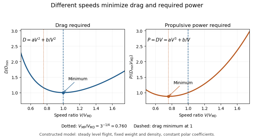
Minimizing required propulsive power instead gives
The minimum-power speed is therefore different from the minimum-drag speed in this model. For stipulated $\rho =1.2kg/{\mathrm{m}}^3$, $S=20{\mathrm{m}}^2$, $W=10000\mathrm{N}$, $C_{D0}=0.020$ and $k=0.050$, the speeds are about $36.30$ and $27.58m/s$, respectively.

These are idealized level-flight comparisons of required propulsive power. Engine efficiency, allowable lift coefficients and a speed-dependent polar can move an operational optimum. Relating the result to minimum sink speed in unpowered flight requires the additional shallow-glide approximation; it does not identify minimum fuel flow for an arbitrary engine.

The minimum-power speed $V_{\mathrm{MP}}$ minimizes the mechanical propulsive power required to sustain the specified flight state. For steady level flight with drag $D(V)$, the required power is $P(V)=D(V)V$, using speed through the air. Minimizing this product is a different problem from finding the minimum-drag speed.

With the fixed-coefficient parabolic drag polar, writeDifferentiation givesThus the stationary point is the unique global minimum for positive speed:At this point, $b/V^2=3a{V}^2$: the decreasing drag contribution is three times the increasing contribution, rather than equal to it. In lift-coefficient form, $C_L^{\mathrm{MP}}=\sqrt{3C_{D0}/k}$.

For an original numerical model with $a=0.20$ and $b=512,000$ in consistent metre-second-newton units, $V_{\mathrm{MD}}=40$ m/s and $V_{\mathrm{MP}}\simeq 30.393$ m/s. The power minimum is about 22.461 kW, with drag about 739.01 N. At the drag minimum, drag is only 640 N but power is 25.600 kW. The lower power comes from the combination of force and speed, despite the greater force.

In shallow steady unpowered descent, the gravitational energy-loss rate approximately balances $DV$, so minimizing required power relates to minimum sink speed when the same assumptions hold. This is consistent with the FAA's distinct minimum-sink and best-glide points.^[ref] A changing propulsive efficiency changes the input-power objective: if $P_{\mathrm{input}}=P/{\eta }_p(V)$, a stationary point satisfies $P^{\prime }/P={\eta }_p^{\prime }/{\eta }_p$, not generally $P^{\prime }=0$.

Attainability must also be checked. The model's optimal lift coefficient can exceed the allowed range before aerodynamic stall. The formula concerns the stated required mechanical power, not a universal minimum of fuel consumption or an operational speed recommendation.

The minimum-drag speed $V_{\mathrm{MD}}$ minimizes the dimensional drag required for steady level flight at fixed gravitational weight, configuration and atmospheric conditions. It is not the speed at the smallest drag coefficient: changing speed changes the dynamic pressure and the lift coefficient needed to support the load.

For the parabolic drag polar $C_D=C_{D0}+k{C}_L^2$, assume $C_{D0}>0$, $k>0$ and constant mass density $\rho$. Substituting $L=W=qS{C}_L$ givesThe ideal finite-wing induced term motivates the quadratic dependence on lift coefficient; a measured whole-aircraft fit needs its own regime assessment.^[ref]

The arithmetic-geometric mean inequality proves a global bound for every $V>0$:Equality holds when $a{V}^2=b/V^2$, so the two modeled drag contributions are equal. Equivalently, the optimum lift coefficient is $C_L^{\mathrm{MD}}=\sqrt{C_{D0}/k}$.

An original model uses $a=0.20$ and $b=512,000$ when $V$ is in m/s and $D$ in newtons. It gives $V_{\mathrm{MD}}=40$ m/s and $D_{\min }=640$ N, with 320 N from each term. At 30 m/s, the terms are 180 and about 568.89 N, giving a larger total of 748.89 N. The slower state nevertheless requires less mechanical power, illustrating the distinct minimum-power speed objective.

At fixed weight, minimizing drag maximizes the lift-to-drag ratio. Under a shallow, steady-glide approximation this relates to best glide through the air, whereas minimum sink speed concerns altitude loss per time. The FAA polar explicitly distinguishes the corresponding operating points.^[ref] Wind, variable coefficients or an unattainable lift coefficient can change the applicable optimum. These model results are not flight instructions or substitutes for measured aircraft performance.