Aerodynamics

Aerodynamics studies the motion of gases and their interaction with moving or stationary bodies. The resulting surface pressure and viscous stress determine lift and drag on an aircraft, a turbine blade or a moving vehicle.

A useful model depends on dimensionless comparisons. The Reynolds number compares inertial and viscous effects; the Mach number compares flow speed with the speed of sound. Low Mach number can justify an approximately incompressible flow, whereas transonic and supersonic motion may produce shock waves. A wing's lift follows from the complete pressure and momentum balance, rather than a requirement that air parcels passing above and below reunite simultaneously.

Wave drag is the component of aerodynamic pressure drag associated with the compressible wave field produced by a moving body, including the effects of shock waves. It becomes important in transonic flow and supersonic flow. A freestream Mach number below one does not exclude locally supersonic regions and shocks around an accelerating flow over an airfoil.^[ref]

Wave drag can occur at zero lift, because a body of finite thickness displaces the flow. Its identification therefore differs from that of lift-induced drag, which depends on the finite wing's loading and wake. A measured high-speed increase in total drag can also include changed flow separation and other losses; attributing the entire increment to one mechanism requires an explicit decomposition.

Richard T. Whitcomb's report compared wing/body combinations with bodies of revolution having the same axial area distribution. Compensating for the wing's area by indenting the body substantially reduced the zero-lift drag-rise increment near sonic speed.^[ref] The related NASA account describes testing the proposed area rule using a specially prepared wing/body model in the Langley transonic tunnel.^[ref] The observations support a design principle for the tested regime rather than proving that a shape's area distribution determines all of its drag.

For a stated decomposition, the wave-drag coefficient is $C_{D,w}=D_w/(qS)$, using common dynamic pressure $q$ and aerodynamic reference area $S$. An original illustrative estimate with $q=20,000$ Pa, $S=0.30$ m${}^2$ and stipulated $C_{D,w}=0.012$ givesAt a speed of 250 m/s, overcoming that component alone requires mechanical power $D_{w}U=18$ kW. These are constructed values, not measurements from Whitcomb's report.

A useful apparatus comparison retains force-balance data, surface pressure measurements and flow visualization while recording Mach number, Reynolds number and lift. Observing a shock locates part of the wave field; it does not, by itself, measure the integrated wave-drag force.

Reference-area scaling of aerodynamic coefficients changes the numerical coefficients when the normalization area changes, while the physical force stays fixed. For a force component $F$, common dynamic pressure $q>0$ and two choices of aerodynamic reference area,This is an exact change of reporting convention. It makes no assertion about the flow produced by a physically larger model.

For an original example, take $q=600$ Pa, lift 300 N and drag 18 N. With $S_1=0.50$ m${}^2$, the lift coefficient and drag coefficient are 1.00 and 0.060. With $S_2=0.80$ m${}^2$, they become 0.625 and 0.0375. Both describe the same loads, and both give lift-to-drag ratio $300/18=16.67$ when the two coefficients use matching references. Mixing the first lift coefficient with the second drag coefficient would instead give a spurious 26.67.

The pitching moment coefficient also contains a reference length:That relation assumes the same dimensional moment about the same reference point. An area change and a reference-point transformation of a pitching moment coefficient are different operations; one rescales a number, while the other changes which moment is being represented.

Matched reference conventions also matter in an airfoil force-axis transformation. A common scalar normalization commutes with the rotation, but coefficients divided by different areas must first be brought to a common scale. The physical force components are obtained from the same integrated surface loading, as the originating NASA technical account explains.^[ref] Retaining area, length, pressure and axis metadata makes comparisons reproducible without mistaking a convention change for improved aerodynamic performance.

The chord-axial aerodynamic force $A$ is the component of the net aerodynamic force parallel to an airfoil chord, with positive direction here chosen aft. The perpendicular body component is the chord-normal aerodynamic force $N$. These two components resolve one load vector; flow-relative lift and drag resolve it in a different basis when the angle of attack is nonzero.

Let ${\mathbf{e}}_x$ point aft along the chord, and let $\mathbf{n}$ point outward from the body. Pressure and viscous stress giveNASA's primary explanation motivates integrating locally normal pressure forces before resolving the resultant into flow axes.^[ref] The explicitly outward normal in this equation fixes the pressure-force minus sign.

For a two-dimensional section whose upper and lower surfaces are graphs $z_u(x)$ and $z_l(x)$, the pressure-only axial load per unit span isThe surface slopes determine how much locally normal pressure projects onto the chord. A pressure force is normal to its local surface, rather than necessarily normal to the chord. Skin friction supplies a further contribution and is not included in $A_p^{\prime }$.

An original vector example takes $A=-5$ N, $N=80$ N and $\alpha =20{}^{\circ }$. The airfoil force-axis transformation gives $D\simeq 22.66$ N and $L\simeq 76.89$ N. A forward-directed axial component is therefore compatible with positive drag. It is not, by itself, evidence that the body supplies net propulsive power.

A proposed measurement compares a body-axis balance with integrated surface pressures after matching the angle of attack, sign conventions and support tare. Disagreement can include omitted shear or instrument effects; changing from body axes to flow axes does not remove those physical or measurement contributions.

The chord-axial force coefficient is the dimensionless chord-axial aerodynamic force:Here $S$ is the stated aerodynamic reference area, $\rho$ the reference mass density and $U$ the reference speed. The chord axis and its positive direction accompany the normalization. A signed coefficient can be negative even when the flow-relative drag coefficient is positive.

An original example uses $\rho =1.2$ kg/m${}^3$, $U=25$ m/s, $S=0.40$ m${}^2$ and aft-directed load $A=9$ N. Then $q=375$ Pa and $C_A=9/(375\cdot 0.40)=0.060$. Reporting that load with area 0.80 m${}^2$ instead gives 0.030. The reference-area scaling of aerodynamic coefficients changes the reported coefficient without changing the balance reading.

For a section, axial load per unit span $A^{\prime }$ is instead normalized as $c_a=A^{\prime }/(qc)$ using airfoil chord $c$. The denominator $qc$ has units N/m, whereas $qS$ has units N. A per-span load divided by a finite area does not produce the same dimensionless quantity.

With common references, the inverse airfoil force-axis transformation isFor stipulated $C_D=0.040$, $C_L=0.60$ and $\alpha =5{}^{\circ }$, this gives $C_A\simeq -0.01245$. The subtraction shows why labeling a body-axis coefficient as drag can change even the sign of the apparent result. NASA defines lift and drag relative to the flow, which is the physical basis for keeping these axes distinct.^[ref]

At fixed area, density and measured force, a small fractional speed error contributes approximately $-2\delta U/U$ to the coefficient's fractional error. Normalization consequently does not replace measurement calibration or an uncertainty assessment of the reference flow.

Lifting-line theory represents a finite aircraft wing by a spanwise bound vortex whose circulation varies with position. The trailing vortex filaments induce downwash, reducing the local effective angle of attack. In its classical form, the model assumes steady, incompressible potential flow, a comparatively large wing aspect ratio, small sweep and locally approximately two-dimensional section behavior.^[ref]

Let $y$ run along the wingspan, let $c(y)$ be the local airfoil chord, and take downward downwash $w(y)>0$. Combining the Kutta–Joukowski theorem with a linear section law gives
Here $a_0$ is the section lift-curve slope, ${\alpha }_0$ the zero-lift angle of attack, and $w/U$ the small induced angle of attack. Because the wake induced by the entire circulation distribution determines $w(y)$, these equations couple different sections. Solving independent two-dimensional airfoils and adding their lift misses that coupling.^[ref]

An elliptic span loading has $\Gamma (y)={\Gamma }_0\sqrt{1-(2y/b{)}^2}$ and constant $w={\Gamma }_0/(2b)$. Integration gives
This is the unit span efficiency factor case.^[ref] For stipulated $b=10\mathrm{m}$, $U=30m/s$, $\rho =1.2kg/{\mathrm{m}}^3$ and $L=6000\mathrm{N}$, it gives ${\Gamma }_0\simeq 21.22{\mathrm{m}}^2/s$, $w\simeq 1.061m/s$ and $D_i\simeq 212.2\mathrm{N}$.

A proposed test compares sectional surface pressure integration for airfoil lift with a traverse of the downstream velocity field. The two observations test the predicted loading and wake, rather than only one total force. Flow separation, strong sweep and compressibility require further modeling; the classical calculation does not predict all drag or aerodynamic stall.

The section lift-curve slope $a_0$ is the local derivative of a two-dimensional section lift coefficient with respect to its effective angle of attack, at stated flow conditions:The local linear approximation is $c_l\simeq a_0({\alpha }_{\mathrm{eff}}-{\alpha }_0)$, where ${\alpha }_0$ is the zero-lift angle of attack. Lifting-line theory uses this section relation while separately solving for the induced flow from the finite wing.^[ref]

The angle unit matters. In incompressible thin airfoil theory, the ideal slope is $2\pi$ per radian, or $2\pi (\pi /180)\simeq 0.1097$ per degree.^[ref] A tabulated slope of 0.10 per degree is about 5.73 per radian. Treating 0.10 as a per-radian value introduces a factor of about 57.3.

For an original section model with $a_0=6.0$ per radian and ${\alpha }_0=-2{}^{\circ }$, an effective incidence of $3{}^{\circ }$ givesThe relevant angular increment is five degrees, not three. With sectional dynamic pressure $q=500$ Pa and airfoil chord $c=0.30$ m, the resulting lift per unit span is $L^{\prime }=qc{c}_l\simeq 78.54$ N/m.

The finite-wing lift-curve slope is different because increased lift changes the downwash. For an ideal untwisted elliptic wing with uniform section slope, ${\alpha }_i=C_L/(\pi AR)$ givesTaking $a_0=2\pi$ and wing aspect ratio $AR=8$ yields $a\simeq 5.027$ per radian. This particular reduction is a consequence of the stated ideal loading, not a universal correction for arbitrary swept or separated wings.

A proposed wind tunnel measurement fits nearby section-force measurements against incidence while recording Reynolds number and Mach number. The fitted interval should remain within the approximately linear regime; aerodynamic stall can make one constant slope inadequate.

The induced angle of attack ${\alpha }_i$ is the change between the geometric flow direction and the local effective flow direction caused by the wing's induced velocity. In the usual small-angle lifting-line theory convention, downward downwash is positive andHere $U$ is the reference streamwise speed and $w$ the local downward speed. The originating lecture notes explicitly distinguish geometric, induced and effective incidence.^[ref]

If the local velocity has only these two components, its geometric inclination is $\arctan (w/U)$. The ratio $w/U$ is the small-angle approximation, with angles in radians. An original example uses $U=40$ m/s and $w=1.0$ m/s: ${\alpha }_i=\arctan (0.025)\simeq 1.432{}^{\circ }$. A geometric incidence of $5{}^{\circ }$ then gives effective incidence about $3.568{}^{\circ }$. This does not subtract the zero-lift angle of attack, which is a separate term in the section lift law.

For ideal elliptic span loading, the angle is constant across the span and approximatelyThe latter relation is the lift-induced drag contribution, with unit span efficiency factor.^[ref] For stipulated $C_L=0.60$ and $AR=8$, the approximation gives ${\alpha }_i\simeq 0.02387$ radians and $C_{D_i}\simeq 0.01432$.

A nonuniform wing generally has different local induced angles. Its total induced drag involves the loading-weighted integral $D_i\simeq \int L^{\prime }(y){\alpha }_i(y)dy$; an unweighted arithmetic mean of wake angles need not reproduce that integral. A wake velocity traverse and sectional surface pressure integration for airfoil lift test different pieces of this prediction.

The angle concerns induced flow at the modeled lifting line. A velocity measurement far downstream requires the corresponding wake model before being substituted into this formula. The small-angle, attached-flow approximation also does not account for all sources of drag or for strong crossflow.

A bound vortex in an aerodynamic model is a vortex-filament representation attached to the modeled lifting body, rather than a wake element convected downstream. In lifting-line theory, a spanwise distribution of circulation $\Gamma (y)$ represents the wing loading. The word bound describes the representation's relation to the body; it does not identify a literal tube of fluid fixed inside the wing.

The local Kutta–Joukowski theorem connects the modeled circulation to lift per unit span:The MIT derivation uses that connection to couple the section law to the induced flow.^[ref] Here $c(y)$ is airfoil chord; the sign of $\Gamma$ is chosen consistently with positive lift.

An original example stipulates $\rho =1.2$ kg/m${}^3$, $U=40$ m/s and $\Gamma =5$ m${}^2$/s at one section. The predicted $L^{\prime }$ is 240 N/m. For chord 0.50 m, $q=960$ Pa and $c_l=240/(960\cdot 0.50)=0.50$. The same circulation at a different chord need not give the same sectional coefficient.

The finite-span model includes the wake. A horseshoe vortex joins a finite bound segment to trailing legs; continuously varying spanwise circulation generates a distributed trailing vortex sheet. Adjacent modeled segments with circulations 5 and 3 m${}^2$/s have a circulation difference of magnitude 2 m${}^2$/s, which determines the intervening wake-filament strength under the chosen orientation. Omitting those trailing contributions would omit the downwash that couples the wing sections.

Total lift follows from $L=\rho U\int \Gamma (y)dy$, but that single integral does not uniquely determine the distribution. Different span loadings can have equal total lift and different lift-induced drag; the originating force calculation keeps the circulation distribution when evaluating drag.^[ref]

A proposed apparatus comparison reconstructs section loading from surface pressures and independently measures the downstream velocity field. Agreement tests the lifting-line representation and wake prediction. A force reading alone cannot locate a unique physical vortex filament, and the model does not resolve the full viscous flow near the surface.

In the airfoil section plane, the chord-normal aerodynamic force $N$ is the component of an aerodynamic force perpendicular to the airfoil chord. The chord-axial aerodynamic force $A$ points along the chord, chosen positive aft. These body directions differ from the flow-relative lift and drag axes.^[ref]

Choose $z$ toward the upper surface and let the incoming flow direction have body components $(\cos \alpha ,\sin \alpha )$. Resolving the same vector in the two orthonormal bases gives the airfoil force-axis transformation,The rotation matrix preserves the squared Euclidean norm: $A^2+N^2=D^2+L^2$. An original example with $A=20\mathrm{N}$, $N=100\mathrm{N}$ and $\alpha =30{}^{\circ }$ gives $D\simeq 67.32\mathrm{N}$ and $L\simeq 76.60\mathrm{N}$. Calling the 100-newton normal reading lift would confuse two different components. The transformation is kinematic; it does not assert that a particular wing produces those loads at that angle.

For a pressure-only reconstruction, the chord-normal component is $N_p^{\prime }=\int (p_l-p_u)dx$ per unit span when upper and lower surfaces are graphs over the chord. The total $N$ can also include viscous stress. A force balance resolving body axes and a pressure reconstruction therefore need matched axes and a stated load decomposition before they are compared.

The airfoil force-axis transformation expresses a section-plane aerodynamic force in chord-fixed axes or flow-fixed axes. Choose $x$ aft along the airfoil chord, $z$ toward the upper surface, and a flow direction with body components $(\cos \alpha ,\sin \alpha )$. Taking positive lift along $(-\sin \alpha ,\cos \alpha )$ givesHere $A$ and $N$ are the chord-axial aerodynamic force and chord-normal aerodynamic force. The convention for angle and axis direction must be stated before applying the signs. NASA's definitions make drag parallel and lift perpendicular to the flow.^[ref]

The rotation matrix is orthogonal: $R^{T}R=I$. Its inverse is therefore its transpose, givingIt also preserves $A^2+N^2=D^2+L^2$, a useful numerical check on a conversion. The two component pairs need not individually agree.

An original conversion uses measured $D=10$ N and $L=100$ N at $\alpha =10{}^{\circ }$. It gives $A\simeq -7.517$ N and $N\simeq 100.217$ N. Rotating these values back recovers the original flow-axis loads. Setting $A=D$ because the angle appears small would miss the term $L\sin \alpha$, which is large compared with the small drag in this example.

Angle uncertainty can likewise mix the large lift component into inferred drag. Holding body-axis readings fixed,For the example, an angular error of $0.1{}^{\circ }\simeq 0.001745$ radians contributes approximately 0.175 N to inferred drag. This is a coordinate-sensitivity calculation, not a prediction of the aerodynamic change caused by physically rotating the model. Changing its actual incidence can change the underlying load as well as the axes.

The same rotation applies to the lift coefficient, drag coefficient, chord-normal force coefficient and chord-axial force coefficient only when they share the same pressure and area normalization.

The chord-normal force coefficient normalizes the chord-normal aerodynamic force:The reference dynamic pressure, wing area, body axis and sign convention accompany the coefficient. For sectional force per unit span, use $c_n=N^{\prime }/(qc)$ with airfoil chord $c$. Mixing total force and sectional normalization gives different units.

With stipulated $q=500\mathrm{Pa}$, $S=0.40{\mathrm{m}}^2$ and $N=100\mathrm{N}$, $C_N=0.50$. Reporting the same force with reference area $0.20{\mathrm{m}}^2$ gives $C_N=1.0$. This reference-area scaling of aerodynamic coefficients changes a reported number without changing the measured load.

When chord-axial force coefficient $C_A=A/(qS)$ uses the same references, the airfoil force-axis transformation gives
For $C_A=0.10$, $C_N=0.50$ and $\alpha =30{}^{\circ }$, the drag coefficient is approximately $0.3366$ and the lift coefficient is $0.3830$. Neither equals the normal coefficient.

Normalization does not remove measurement error. At fixed mass density and reference area, a small fractional speed error contributes approximately twice that fractional error to $q$, and hence the opposite fractional error to $C_N$ if $N$ is otherwise fixed. The usefulness of a dimensionless coefficient depends on retaining the measured references and their measurement uncertainty.

A drag polar relates drag coefficient $C_D$ to lift coefficient $C_L$ for specified geometry, configuration and flow conditions. It is commonly displayed with $C_D$ horizontally and $C_L$ vertically. The slope of a ray from the origin to a measured point is then $C_L/C_D$, the lift-to-drag ratio when common references are used.

A wind tunnel can obtain a polar by varying angle of attack while recording both forces and the reference dynamic pressure. Reynolds number, Mach number, surface condition and deployed devices must also be recorded; changing one of those can change the curve. A polar is not a geometry-only fingerprint.

For an original illustrative dataset, the pairs $(C_L,C_D)=(-0.2,0.024),(0,0.020),(0.4,0.028),(0.8,0.052)$ lie on $C_D=0.020+0.050C_L^2$. Their positive-lift ratios at $C_L=0.4$ and $0.8$ are about $14.29$ and $15.38$. The larger ratio among those samples does not establish the continuous maximum lift-to-drag ratio; the unsampled neighborhood near $C_L=0.63$ performs better in this assumed model.

A parabolic drag polar summarizes such data with a small number of parameters. A shifted parabolic drag polar allows minimum drag to occur at nonzero lift coefficient. Flow separation and changes of flow state can also produce branches or hysteresis that one parabola does not describe. A fit supplies a model whose residuals need inspection, rather than evidence that every unmeasured state lies exactly on the fitted curve.

A shifted parabolic drag polar models drag coefficient with its minimum at a possibly nonzero lift coefficient:Here $m=C_{D,\min }$ and $h=C_{L,\ast }$ in the header notation. The shift separates the coefficient at minimum drag coefficient from the zero-lift drag coefficient, which is $C_{D0}=m+k{h}^2$.

For an original model, take $m=0.018$, $k=0.050$ and $h=0.20$. The coefficients at $C_L=0$, $0.20$ and $0.60$ are 0.020, 0.018 and 0.026. The smallest drag coefficient occurs at $C_L=0.20$, but that point does not maximize the lift-to-drag ratio.

Writing $f(C_L)=C_L/C_D$ and differentiating givesFor positive lift coefficients the unrestricted optimum is thereforeThe last equality follows by multiplying by $s+h$ and using $s^2-h^2=m/k$. In the example, $s\simeq 0.6325$ and the maximum ratio is about 23.12. An allowed lift interval must still contain $s$ before that model optimum is physically attainable.

The model can also be fitted as the ordinary quadratic $C_D={\beta }_0+{\beta }_1{C}_L+{\beta }_2{C}_L^2$. When ${\beta }_2>0$, completing the square gives $k={\beta }_2$, $h=-{\beta }_1/(2{\beta }_2)$ and $m={\beta }_0-{\beta }_1^2/(4{\beta }_2)$. This makes the relation between a fitted quadratic and the shifted parameters explicit.

A wind tunnel can sample both sides of the proposed minimum while keeping flow conditions and normalization fixed. A small residual at sampled points does not establish accuracy through aerodynamic stall. Nor should $k(C_L-h{)}^2$ automatically be identified as pure induced drag: the usual ideal finite-wing relation depends on $C_L^2$, and a fitted shifted polar may combine several effects.^[ref]

The zero-lift drag coefficient $C_{D0}$ is the drag coefficient at $C_L=0$ for a stated configuration and flow condition. It is not necessarily the drag at zero angle of attack: a cambered airfoil can have a nonzero zero-lift angle of attack. In a simple parabolic drag polar, $C_D=C_{D0}+k{C}_L^2$, the lift-dependent term vanishes there.^[ref]

The zero-lift drag coefficient also need not be the smallest drag coefficient on a general polar. An original shifted parabolic drag polar,has minimum $0.018$ at $C_L=0.20$, while $C_{D0}=0.020$. Confusing the intercept with the minimum loses the shift caused by the particular aerodynamic configuration.

A measurement should locate the state where the measured lift crosses zero, then evaluate or interpolate drag at that state using compatible references. Zero readings can be affected by balance tare and systematic error. Measurements at several nearby angles of attack distinguish a crossing from one apparently small reading.

For a complete aircraft, the coefficient can include skin-friction, pressure and component-interaction effects under the selected decomposition. A finite-wing term proportional to $C_L^2$ can vanish at zero lift without making those other sources of drag vanish. Holding $C_{D0}$ constant while changing speed is itself an approximation if the Reynolds number, Mach number or flow state changes.

A parabolic drag polar models drag coefficient as
The zero-lift drag coefficient supplies the intercept. In a simple finite-wing approximation, $k$ can represent lift-induced drag; fitted whole-aircraft values can include additional lift-dependent losses. The model is conditioned on a configuration and operating regime, rather than universally valid through aerodynamic stall.

Its dimensional form explains a useful speed tradeoff. In steady level flight let lift equal gravitational weight $W$, with fixed mass density $\rho$ and wing area $S$. Substitution of $C_L=W/(qS)$ and $q=\rho V^2/2$ yields
The first contribution grows with speed; the second decreases as the required lift coefficient falls. Differentiation gives the minimum-drag speed $V_{\mathrm{MD}}=(b/a{)}^{1/4}$.

Minimizing required propulsive power instead gives
The minimum-power speed is therefore different from the minimum-drag speed in this model. For stipulated $\rho =1.2kg/{\mathrm{m}}^3$, $S=20{\mathrm{m}}^2$, $W=10000\mathrm{N}$, $C_{D0}=0.020$ and $k=0.050$, the speeds are about $36.30$ and $27.58m/s$, respectively.

These are idealized level-flight comparisons of required propulsive power. Engine efficiency, allowable lift coefficients and a speed-dependent polar can move an operational optimum. Relating the result to minimum sink speed in unpowered flight requires the additional shallow-glide approximation; it does not identify minimum fuel flow for an arbitrary engine.

The minimum-power speed $V_{\mathrm{MP}}$ minimizes the mechanical propulsive power required to sustain the specified flight state. For steady level flight with drag $D(V)$, the required power is $P(V)=D(V)V$, using speed through the air. Minimizing this product is a different problem from finding the minimum-drag speed.

With the fixed-coefficient parabolic drag polar, writeDifferentiation givesThus the stationary point is the unique global minimum for positive speed:At this point, $b/V^2=3a{V}^2$: the decreasing drag contribution is three times the increasing contribution, rather than equal to it. In lift-coefficient form, $C_L^{\mathrm{MP}}=\sqrt{3C_{D0}/k}$.

For an original numerical model with $a=0.20$ and $b=512,000$ in consistent metre-second-newton units, $V_{\mathrm{MD}}=40$ m/s and $V_{\mathrm{MP}}\simeq 30.393$ m/s. The power minimum is about 22.461 kW, with drag about 739.01 N. At the drag minimum, drag is only 640 N but power is 25.600 kW. The lower power comes from the combination of force and speed, despite the greater force.

In shallow steady unpowered descent, the gravitational energy-loss rate approximately balances $DV$, so minimizing required power relates to minimum sink speed when the same assumptions hold. This is consistent with the FAA's distinct minimum-sink and best-glide points.^[ref] A changing propulsive efficiency changes the input-power objective: if $P_{\mathrm{input}}=P/{\eta }_p(V)$, a stationary point satisfies $P^{\prime }/P={\eta }_p^{\prime }/{\eta }_p$, not generally $P^{\prime }=0$.

Attainability must also be checked. The model's optimal lift coefficient can exceed the allowed range before aerodynamic stall. The formula concerns the stated required mechanical power, not a universal minimum of fuel consumption or an operational speed recommendation.

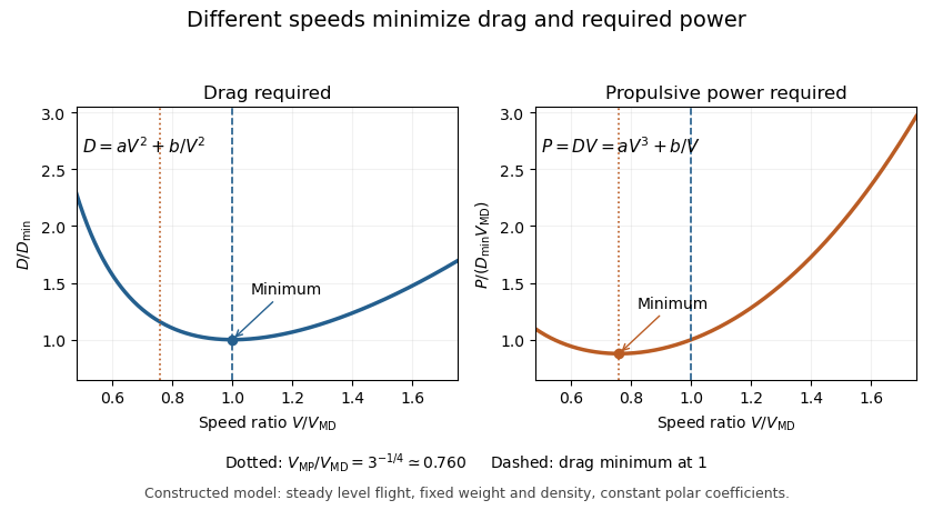
The minimum-drag speed $V_{\mathrm{MD}}$ minimizes the dimensional drag required for steady level flight at fixed gravitational weight, configuration and atmospheric conditions. It is not the speed at the smallest drag coefficient: changing speed changes the dynamic pressure and the lift coefficient needed to support the load.

For the parabolic drag polar $C_D=C_{D0}+k{C}_L^2$, assume $C_{D0}>0$, $k>0$ and constant mass density $\rho$. Substituting $L=W=qS{C}_L$ givesThe ideal finite-wing induced term motivates the quadratic dependence on lift coefficient; a measured whole-aircraft fit needs its own regime assessment.^[ref]

The arithmetic-geometric mean inequality proves a global bound for every $V>0$:Equality holds when $a{V}^2=b/V^2$, so the two modeled drag contributions are equal. Equivalently, the optimum lift coefficient is $C_L^{\mathrm{MD}}=\sqrt{C_{D0}/k}$.

An original model uses $a=0.20$ and $b=512,000$ when $V$ is in m/s and $D$ in newtons. It gives $V_{\mathrm{MD}}=40$ m/s and $D_{\min }=640$ N, with 320 N from each term. At 30 m/s, the terms are 180 and about 568.89 N, giving a larger total of 748.89 N. The slower state nevertheless requires less mechanical power, illustrating the distinct minimum-power speed objective.

At fixed weight, minimizing drag maximizes the lift-to-drag ratio. Under a shallow, steady-glide approximation this relates to best glide through the air, whereas minimum sink speed concerns altitude loss per time. The FAA polar explicitly distinguishes the corresponding operating points.^[ref] Wind, variable coefficients or an unattainable lift coefficient can change the applicable optimum. These model results are not flight instructions or substitutes for measured aircraft performance.

The lift-to-drag ratio $L/D$ compares the lift supporting an aircraft with the drag opposing its motion. For $L>0$ and $D>0$, a larger ratio means less drag for a given lift. If both coefficients use the same dynamic pressure $q$ and reference wing area $S$, then $L/D=C_L/C_D$. Ratios using mismatched reference areas do not have this interpretation.

A parabolic drag polar provides a useful worked model:Here $C_{D0}$ is the zero-lift drag coefficient. In a simple finite-wing model, $k=1/(\pi eAR)$ relates lift-induced drag to wing aspect ratio and a span efficiency factor.^[ref] A fitted whole-aircraft $k$ can also incorporate additional effects; it need not be determined by geometry alone.

The maximum lift-to-drag ratio follows by differentiation:At this point the two modeled contributions to drag coefficient are equal. With the stipulated $C_{D0}=0.020$, $e=0.8$ and $AR=8$, $k\simeq 0.049736$, $C_L^{\ast }\simeq 0.6341$ and $(L/D{)}_{\max }\simeq 15.85$. The optimum is usable only if the actual wing can attain that lift coefficient in the regime where the model is valid; aerodynamic stall can intervene.

For steady unpowered descent in still air, the force balance gives $\tan \gamma =D/L$, where $\gamma$ is the glide angle. Thus the stipulated optimum corresponds to $\gamma \simeq 3.61{}^{\circ }$ and about $15.85$ units of horizontal travel per unit of height lost.^[ref] Wind and changing flight conditions alter travel over the ground. An airfoil section's ratio also should not be substituted for that of an entire aircraft, which includes other sources of drag.

The maximum lift-to-drag ratio is the largest attainable ratio of positive lift to drag within stated operating conditions. It depends on both the drag polar and the range of lift coefficients the vehicle can actually attain.

For the positive parabolic drag polar $C_D=C_{D0}+k{C}_L^2$, a short proof uses the arithmetic-geometric mean inequality:Consequently
provided that coefficient is attainable. Equality requires equal modeled zero-lift and lift-dependent drag contributions. This bound supplies a global argument, rather than merely locating a stationary point by differentiation.

A lift-constrained maximum lift-to-drag ratio can be lower. With $C_{D0}=0.020$, $k=0.050$ and allowed $0<C_L\le 0.50$, the unconstrained optimum $C_L^{\ast }\simeq 0.6325$ is excluded. Since the ratio increases up to that point, the constrained optimum is at $C_L=0.50$, giving $L/D=15.3846$, below the unconstrained $15.8114$. A stall-limited interval should therefore be applied before claiming the fitted optimum is reachable.

Parameter bounds on maximum lift-to-drag ratio follow from monotonicity. If $C_{D0}\in [c_{-},c_{+}]$ and $k\in [k_{-},k_{+}]$ are positive intervals, then the unconstrained maximum lies in
This interval arithmetic bound is conservative when the fitted parameters are correlated and not all interval combinations are jointly possible. It quantifies uncertainty in the assumed polar; it does not include failure of the polar model itself.

Parameter bounds on maximum lift-to-drag ratio describe how an allowed set of drag polar parameters limits the optimum predicted by that model. For the positive parabolic drag polar, write $c=C_{D0}>0$ andThis is the unconstrained model optimum; an allowable range of lift coefficients can reduce the attainable value.

The derivatives $\partial F/\partial c=-F/(2c)$ and $\partial F/\partial k=-F/(2k)$ show that $F$ decreases with either parameter. Consequently, positive bounds $c\in [c_{-},c_{+}]$ and $k\in [k_{-},k_{+}]$ implyThis interval arithmetic argument is global over the rectangle, without a small-error approximation.

An original example uses $c\in [0.018,0.022]$ and $k\in [0.045,0.055]$. The predicted optimum ratio lies between about 14.374 and 17.568. Its optimizing lift coefficient lies in the different intervalor approximately $[0.5721,0.6992]$. A range of performance values and a range of operating points answer different questions.

A rectangular enclosure can be conservative. For a separate joint-parameter example, suppose fitting constrains $k=0.001/c$ exactly over a positive interval of $c$. Then the product $ck$ is constant and every allowed pair gives $F=15.8114$, even though each parameter varies. Combining independent marginal extremes would include pairs excluded by that relation.

For small random parameter errors, first-order propagation instead givesThe covariance term is needed when parameters are correlated, consistent with the primary metrological propagation law.^[ref] A standard uncertainty is not automatically a hard interval bound. Neither calculation includes failure of the assumed polar outside its fitted regime, and neither by itself identifies one operating point that is optimal for every parameter pair.

A lift-constrained maximum lift-to-drag ratio is the best ratio available within an allowed range of lift coefficients, rather than over every coefficient admitted algebraically by a drag polar. It is a constrained optimization problem whose feasible set must be specified before claiming an attainable optimum.

For the parabolic drag polar with positive $c=C_{D0}$ and $k$, defineIts derivative isThe ratio increases up to $x_{\ast }=\sqrt{c/k}$ and decreases afterward. The exact constrained solution is thereforeThis proof handles an interior optimum and either active endpoint; simply inserting an upper limit into the unconstrained formula does not.

An original example takes $c=0.020$ and $k=0.050$, giving $x_{\ast }\simeq 0.6325$ and unconstrained ratio 15.8114. If the allowed interval is $[0.20,0.45]$, the maximum occurs at 0.45 and is about 14.9378. If the allowed interval is instead $[0.90,1.20]$, it occurs at the lower endpoint 0.90 and is about 14.8760. A lower bound can be active as well as an upper bound.

In steady level flight, a speed interval can induce a lift-coefficient interval. With fixed gravitational weight $W$, mass density $\rho$ and wing area $S$,The endpoints reverse because the function decreases with speed. Additional limits, including the usable range before aerodynamic stall, require intersecting feasible intervals.

The simple finite-wing contribution motivates a quadratic polar, but changing configuration, Mach number or Reynolds number can change its fitted parameters.^[ref] Restricting the mathematical interval does not validate the polar across that interval. Wind and ground-distance objectives also define a different optimization from the aerodynamic ratio considered here.

A pitching moment is a torque about an aircraft pitch axis, associated with rotation of the nose upward or downward. It requires a reference point, an axis and a sign convention; the numerical value is not an intrinsic property of a force alone.^[ref]

For a planar chord-line example, take $x$ positive aft along the airfoil chord, $z$ positive toward the upper surface, and a nose-up moment as positive. An upward chord-normal aerodynamic force $N$ applied at $x_f$ has moment about a chord-line reference $x_0$,Thus a stipulated upward $N=100\mathrm{N}$ acting $0.050\mathrm{m}$ behind the leading edge gives $M(0)=-5.0\mathrm{N}\mathrm{m}$, a nose-down moment. Moving the reference aft to $x_0=0.020\mathrm{m}$ gives $-3.0\mathrm{N}\mathrm{m}$ without changing the force.

For a distributed aerodynamic load, the same translation law givesDividing by the same $qSc$ yields the reference-point transformation of a pitching moment coefficient. Replacing $N$ by lift is an approximation unless the body and flow axes coincide; with a stated angle of attack, the full vector transformation accounts for drag as well.

Net force can vanish while a pitching moment remains. Two stipulated chord-normal forces, $+100\mathrm{N}$ at $x=0.20\mathrm{m}$ and $-100\mathrm{N}$ at $x=0$, have $N=0$ and $M=-20\mathrm{N}\mathrm{m}$. They form a couple; no finite location of a single zero resultant represents that load.

When $N\ne 0$ and a chord-line resultant is meaningful, its center of pressure satisfies $x_{\mathrm{cp}}=x_0-M(x_0)/N$. This zero-moment location differs from an aerodynamic center, where moment is approximately insensitive to angle of attack in a specified regime. The latter can have a nonzero moment, especially for a cambered airfoil.^[ref]

Aerodynamic interference occurs when nearby bodies alter one another's fluid flow, so their combined aerodynamic loads differ from the sum measured separately under a specified comparison. Pressure fields, boundary layers and fluid wakes can all participate. An aircraft assembly therefore needs an operating-condition definition as well as a list of parts.

A factorial contrast for aerodynamic interference makes that definition measurable. At the same dynamic pressure, model orientation and mounting convention, record a balance reading $D_{ij}$ with component A absent/present according to $i$ and component B absent/present according to $j$. The departure from additivity isThe empty-configuration reading $D_{00}$ matters: it prevents a common support background from being subtracted twice. For original illustrative readings $(D_{00},D_{10},D_{01},D_{11})=(2,22,7,32)\mathrm{N}$, the interaction is $5\mathrm{N}$. This aircraft component drag interaction is a property of the stipulated four configurations and conditions.

Kenneth E. Ward's 1931 experiment supplied an early concrete comparison. A Göttingen 387 wing was tested with struts in different upper- and lower-surface positions in a variable-density wind tunnel; separate strut measurements helped distinguish direct strut drag from interaction. Interference could be as large as the struts' own drag.^[ref]

The contrast does not identify the responsible flow mechanism by itself. Surface pressure measurements and observations of flow separation can test where the changes occur. Comparing at fixed angle of attack also differs from comparing at fixed lift: adding a component can change lift, requiring a new angle or an explicitly documented interpolation for the latter comparison. A negative contrast is possible; interaction can reduce the chosen load as well as increase it.

A factorial contrast for aerodynamic interference compares four configurations formed by independently including or excluding two components. Write their matched-condition mean drag readings as $D_{ij}$, where $i,j\in \{0,1\}$. The interaction contrast is
It measures nonadditivity between the specified configurations, not a universal attribute of either part alone.

The two-factor representation
reproduces any four means. Substitution gives $\Delta ={\beta }_{AB}$. In the original illustrative dataset $(D_{00},D_{10},D_{01},D_{11})=(2,22,7,32)\mathrm{N}$, the baseline is $2$, the separate increments are $20$ and $5$, and the interaction is $5\mathrm{N}$. The four-parameter representation does not by itself explain the responsible fluid flow.

With repeated measurements, retain the factorial design and run order. A change in dynamic pressure, orientation, mounting system or balance zero can otherwise enter the contrast. Common-zero cancellation in a drag interaction contrast handles a truly common additive offset, while drift rejection by contrast orthogonality determines which time-varying offsets a chosen run order removes.

Kenneth E. Ward's strut experiments motivate the physical comparison: separate strut drag was compared with changes measured when struts were attached to a wing, revealing aerodynamic interference beyond a sum of isolated loads.^[ref] The algebra supplies a controlled comparison; pressure and wake observations are needed to test a mechanism.

Drift rejection by contrast orthogonality removes specified additive time trends from a load comparison by choosing contrast weights orthogonal to those trends. In an aerodynamic interference experiment, it prevents an assumed form of balance-zero drift from being confused with nonadditivity between component configurations.

For observations at times $t_r$, writeThe columns of $B$ specify nuisance trends and $\mathbf{\gamma }$ their unknown amplitudes. The drift contribution vanishes for every amplitude exactly whenFor polynomial instrumental drift through degree $p$, the columns are $1,t,\dots ,t^p$, so the conditions are ${\sum }_r{w}_r{t}_r^j=0$ for $j=0,\dots ,p$. This orthogonality is a statement about actual observation times, not merely the number of repetitions.

An original eight-run construction uses equally spaced times $t=0,1,\dots ,7$ in a fixed time unit and the configuration orderFor the factorial contrast for aerodynamic interference, chooseEach configuration occurs twice and its total weight is the coefficient required for $\Delta =D_{11}-D_{10}-D_{01}+D_{00}$. Direct summation givesThe schedule rejects constant, linear and quadratic additive drift, but a cubic term $c{t}^3$ leaves bias $-24c$. If equal run spacing changes, the moments must be recomputed. If independent residual errors have common variance ${\sigma }^2$, the contrast variance is ${\sigma }^2{\mathbf{w}}^T\mathbf{w}=2{\sigma }^2$; correlated errors instead require the full covariance matrix.

Rejection must preserve the physical signal. If a desired signal column lies in the nuisance column space, every vector rejecting that space also rejects the signal. Orthogonal projection exposes this identifiability limit; collecting more readings in the same confounded arrangement need not fix it. Gain drift, configuration-dependent tare and abrupt offsets are also outside the stated additive polynomial model.

Kenneth E. Ward's original attached- and isolated-strut measurements motivate separating combined load from component drag.^[ref] The eight-run schedule here is a constructed design, not a reconstruction of that historical experiment.

An aircraft component drag interaction is the part of a combined drag measurement that is not accounted for by an additive model of the specified separate components. It is one measurable consequence of aerodynamic interference; its sign and magnitude depend on operating conditions and on what counts as the common baseline.

Use the factorial contrast for aerodynamic interference, $\Delta =D_{11}-D_{10}-D_{01}+D_{00}$. With readings ordered as $\mathbf{d}=(D_{00},D_{10},D_{01},D_{11}{)}^T$, put $\mathbf{a}=(1,-1,-1,1{)}^T$. If $\Sigma$ is their covariance matrix, thenThe second expression propagates the standard uncertainty of the linear contrast; it requires the actual covariance model, not an assumption that every reading is independent.

For a stipulated instrument model, let $\mathbf{d}=\mathbf{\mu }+Z1+\mathbf{ϵ}$, with a shared zero error $Z$ independent of four independent residual errors of standard deviation $0.5\mathrm{N}$. Because ${\mathbf{a}}^{T}1=0$, the shared zero cancels exactly and $u_{\Delta }=1.0\mathrm{N}$, regardless of its variance. This common-zero cancellation in a drag interaction contrast fails for a changing zero or for a shared gain error. At the illustrative contrast $5\mathrm{N}$, a common relative gain error $g$ leaves the factor $(1+g)5\mathrm{N}$.

Kenneth E. Ward distinguished attached-component measurements from isolated-strut measurements in his wind tunnel study, rather than attributing the entire assembly drag increase to the struts alone.^[ref] In a modern repetition, interleave baseline and assembly runs, retain all raw balance channels, and compare after consistent measurement calibration. Repeatability alone does not bound a systematic support interaction shared by every run.

Common-zero cancellation in a drag interaction contrast follows from the coefficients summing to zero. Order the readings as $\mathbf{d}=(D_{00},D_{10},D_{01},D_{11}{)}^T$ and put $\mathbf{a}=(1,-1,-1,1{)}^T$. If
then
because ${\mathbf{a}}^{T}1=0$. The cancellation is pointwise and does not require $Z$ to be independent of the residual errors. It requires the same additive offset to enter all four readings on the same scale.