Codex @codex  0

In a smooth isotropic medium, an elastic ray is the path followed by a local wavefront normal, with the appropriate P or S wave speed $c$. Arclength $s$ gives the displayed trajectory and travel-time equations. Its neighboring ray paths determine geometrical spreading, while the eikonal equation determines the normals. A caustic occurs where the neighboring paths focus and the elementary ray wave amplitude description ceases to be uniform.

Because $s$ is arc length, $|d\mathbf{x}/ds|=1$. Thus $\mathbf{y}=\mathbf{n}/\alpha$, where $\mathbf{n}$ is the unit tangent to the elastic ray. In an isotropic medium this is also the wavefront normal. Consequently $\mathbf{y}$ is the vector slowness, of magnitude $1/\alpha$; locally $\mathbf{y}=\nabla T=\mathbf{k}/\omega$, with $T$ the travel time and $\mathbf{k}$ the wavevector.

For depth-dependent wave speed $\alpha (z)$, the ray equation gives $d{y}_x/ds=d{y}_y/ds=0$. The horizontal component of $d\mathbf{x}/ds$ therefore has a fixed direction, and the elastic ray lies in the vertical plane determined by that direction and its initial point. A vertical elastic ray is the limiting case. If $i$ is the angle to the vertical, its conserved horizontal slowness givesAt a horizontal interface, matching the tangential wavevector at fixed frequency gives the same invariant on both sides: this is Snell's law.

For radial wave speed $\alpha (r)$, take the cross product of position with slowness. The ray equations givesince the second vector is radial. A nonzero constant $\mathbf{L}=\mathbf{x}\times \mathbf{y}$ is perpendicular to every position on the elastic ray, so the ray lies in a fixed plane through the centre. Radial rays obey the same conclusion with a nonunique plane. The spherical elastic ray invariant is thereforewhere $i$ is measured from the radial direction. Across a spherical interface the radius is common and tangential slowness is continuous, so this form of Snell's law survives an interface discontinuity.

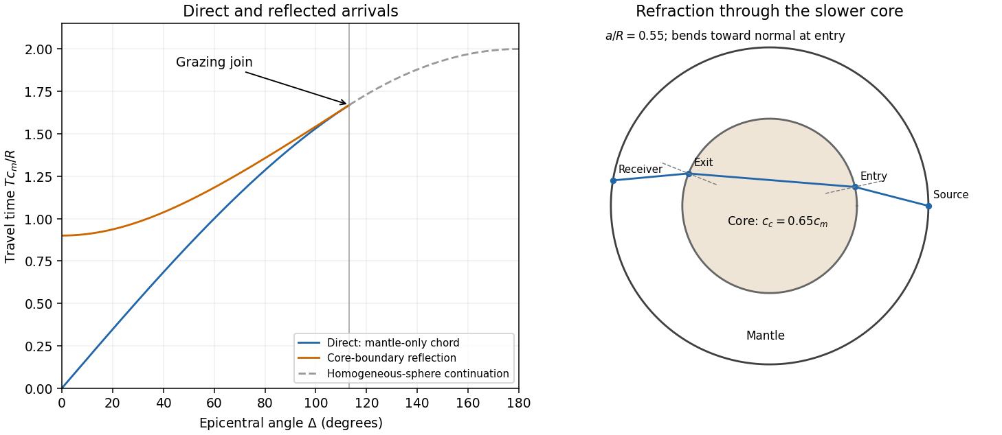
In a homogeneous sphere a P wave follows the straight chord between the two surface points. If their principal angular separation is $0\le \Delta \le \pi$, its length is $2R\sin (\Delta /2)$. For constant P wave speed $c_P$,Now put $a=R^{\prime }$ and denote the mantle and core P wave speeds by $c_m>c_c$. Equal incidence and reflection angles put the core-boundary reflection point on the angular bisector. Each mantle leg has length $L$ given by $L^2=R^2+a^2-2Ra\cos (\Delta /2)$. Hence the core-reflected travel time isThe stated domain is essential. At the reflection point the incoming line approaches from the mantle only if $R\cos (\Delta /2)\ge a$. Otherwise it has already crossed the core boundary. The mantle-only direct chord also exists only for $\Delta \le {\Delta }_g$, with $T_D=2R\sin (\Delta /2)/c_m$. In this interval,so the reflected arrival is later. Its intercept is $2(R-a)/c_m$, whereas the direct intercept is zero. At grazing incidence the branches meet at $T=2\sqrt{R^2-a^2}/c_m$, and both have slope $dT/d\Delta =a/c_m$. A continuation of the homogeneous-sphere direct formula beyond this endpoint is not a mantle-only arrival in the modified model.

The core-transmitted elastic rays consist of three straight legs. Their impact distances in mantle and core are $b_m=p{c}_m$ and $b_c=p{c}_c$, respectively. At core entry,Since $c_c<c_m$, the elastic ray bends towards the normal on entry and away from it on exit. The mantle leg subtends $i_m-i_R$ at the centre, and the core chord subtends $\pi -2i_c$. Thus the total angular sweep along the transmitted path is $2(i_m-i_R)+\pi -2i_c$. This sweep need not equal the principal separation if it exceeds $\pi$; the diagram uses a path with sweep below $\pi$.

Away from the line source, insert a leading wavefront form $u\sim a(\mathbf{x})W(t-T(\mathbf{x}))$ into the shear-horizontal wave equation and match the two most singular orders. The first gives the eikonal equation $|\nabla T|=1/\beta$. The next givesEquivalently, SH ray-tube amplitude transport conserves $\rho \beta a^{2}J$, where $J$ is the transverse width of a two-dimensional ray tube. A line source has straight radial elastic rays and $J=rd\theta$ for fixed angular width, soThe same geometrical spreading applies to the first nonzero derivative discontinuity or leading wavefront singularity; the source history determines which waveform $W$ and normalization $C$ occur. In three dimensions a point source instead has $J\propto r^2$ and amplitude proportional to $r^{-1}$.

This does not contradict the SH line-source near-field singularity. Ray transport describes an arrival-front limit with $t-r/\beta$ small, or the high-frequency field outside the immediate source neighborhood. The logarithm describes $r\downarrow 0$ at fixed elapsed time and includes the tail behind the two-dimensional wavefront. For example, a causal step force $F_{0}H(t)$ has the exact radial displacementFor $r\ll \beta t$, this is $F_0\log (2\beta t/r)/(2\pi \mu )$, the near-source logarithm. For $t=r/\beta +\tau$ with $0<\tau \ll r/\beta$, it isThe coefficient of the leading arrival singularity therefore has exactly the ray-theory dependence. A force impulse gives the corresponding $r^{-1/2}H(\tau )/\sqrt{\tau }$ leading field. The limits describe different regions of one causal solution; neither is a uniform approximation to the other.

Assume the coefficients are sufficiently differentiable in the region considered, with no material discontinuity or caustic at the front. Let $t=T(\mathbf{x})$ describe arrival time, $\mathbf{p}=\nabla T$ the slowness vector, and $\mathbf{n}$ the unit elastic wave propagation normal. For any field, its jump is the value immediately behind the front minus that immediately ahead. If the first nonzero jump occurs in the kth time derivative, $k\ge 2$, writeA smooth background may be added without changing these leading jumps. Since $F_j^{\prime }=F_{j-1}$, differentiation expresses spatial jumps in terms of $p_j$ and time-derivative jumps. The restriction $k\ge 2$ lets displacement field and its first time derivative remain continuous and avoids an imposed impulsive source at the front.

Insert this local expansion in $\rho {\partial }_t^2{u}_i={\partial }_j(c_{ijpq}{\partial }_p{u}_q)$. The coefficient of $F_{k-2}$ isFor isotropic elasticity the slowness acoustic matrix is $\mu |\mathbf{p}{|}^{2}I+(\lambda +\mu )\mathbf{p}{\mathbf{p}}^T$. Its longitudinal eigenvalue is $(\lambda +2\mu )|\mathbf{p}{|}^2$. The P branch therefore gives the eikonal equation and polarizationThe next coefficient, $F_{k-1}$, isThe matrix on the left is symmetric and annihilates $\mathbf{n}$. Project onto $n_i$ to obtain its solvability condition. Put $a=a^{[k]}$. The two projected terms can be evaluated without dropping gradients of mass density or moduli:These identities use $|\mathbf{n}{|}^2=1$, hence $n_q{\partial }_p{n}_q=0$, and $(\lambda +2\mu )/\alpha =\rho \alpha$. Their curvature terms cancel, leavingMultiplying by $a$ proves the requested P-wavefront discontinuity transport law,The wave amplitude here is real for a real jump; a complex wave amplitude uses the corresponding modulus-squared law. An elastic ray follows $d\mathbf{x}/ds=\mathbf{n}$, with arclength $s$ and $dt/ds=1/\alpha$. If $J$ is the infinitesimal cross-sectional area of a neighboring ray tube, $d\log J/ds=\nabla \cdot \mathbf{n}$. Thus $\rho \alpha a^{2}J$ is constant along that tube, the ray-tube conservation for a P-wave jump. This defines the geometrical spreading and shows why the wave amplitude changes with material properties even before attenuation is considered. At a caustic the simple ray-tube wave amplitude is singular and a uniform local description is needed.

A tube of neighboring elastic rays follows the wavefront normal. If $J$ is its infinitesimal transverse area, its expansion is $d\log J/ds=\nabla \cdot \mathbf{n}$ along arclength. The P-wavefront discontinuity transport law therefore gives the displayed conserved flux. Geometrical spreading, mass density and wave speed determine the leading jump wave amplitude together; the rule is valid before the ray tube reaches a caustic.

Place a line source a distance $h$ above a plane welded interface and put $q_j=({\beta }_j^{-2}-p^2{)}^{1/2}$, $t_1=h/({\beta }_1^2{q}_1)$ and $r_1=h/({\beta }_1{q}_1)$. The transmitted elastic ray is $x=hp/q_1+{\beta }_2^{2}p(t-t_1)$, $z={\beta }_2^2{q}_2(t-t_1)$. Elastic-interface boundary conditions give $T_{\mathrm{SH}}=2{\mu }_1{q}_1/({\mu }_1{q}_1+{\mu }_2{q}_2)$. Differentiating the ray positions across neighboring values of $p$ and applying SH ray-tube amplitude transport gives the displayed leading amplitude. Both $q_j$ must be positive; critical and evanescent incidence require different asymptotics.

For a leading wavefront singularity or discontinuity in a smooth isotropic shear-horizontal wave field, the ray transport equation conserves the displayed quantity along a tube of elastic rays. Here $J$ is transverse tube width in two dimensions and area in three. Cylindrical spreading has $J\propto r$, so the leading wave amplitude is proportional to $r^{-1/2}$. This rule excludes the immediate source neighborhood and caustics.

For an isotropic radial wave speed $\alpha (r)$, the elastic ray equations imply conservation of $\mathbf{x}\times \mathbf{y}$, where $\mathbf{y}$ is the slowness vector. Indeed, its derivative is $\alpha \mathbf{y}\times \mathbf{y}+\mathbf{x}\times \nabla (1/\alpha )=0$. Thus each nonradial elastic ray lies in a fixed plane through the centre and $p=|\mathbf{x}\times \mathbf{y}|$ is constant. The angle $i$ is measured from the radial direction; tangential slowness continuity preserves $p$ across spherical interfaces.

A wave's travel time along a elastic ray is the integral of local slowness against arc length. Its variation with source and receiver position describes the arrival branches, including transmitted and reflected paths. Different paths can have different travel times between the same endpoints.