Elasticity studies reversible deformation and the stresses produced by it.
The boundary of the loading range within which a material recovers its original configuration on unloading. Elasticity need not be linear; beyond the elastic range, permanent plastic deformation or damage may remain.
Failure by crack formation or propagation with limited distributed permanent deformation. Shear and opening fractures have different strength conditions; a frictional failure envelope should not be extrapolated indefinitely into tension.
Loss of load-bearing strength accompanied by relative displacement tangential to a surface, rather than primarily opening normal to it. The Mohr-Coulomb failure criterion models frictional shear failure by , using cohesion, a friction coefficient and compressive effective stress normal to the potential sliding plane.
In the simplest strength-cutoff model, opening begins when the least compressive effective stress reaches minus the tensile strength: with compression positive. In Mohr's circle, this is contact with the vertical line at . The criterion represents an opening mechanism and differs from frictional shear failure.
A coefficient relating an appropriate stress and strain in the linear elastic regime. Young's modulus, shear modulus and bulk modulus describe different deformation modes.
Loss of stability of a loaded configuration toward a bent or folded form. The threshold and deformation mode depend on geometry, material properties and boundary conditions.
A flat, unsupported film's bending and tension energies give modal stiffness . Negative tension represents compression, destabilizing sufficiently long waves. A finite sheet restricts allowed wave numbers, while a supporting foundation adds stiffness and can select a wrinkle wavelength. This is generic continuum mechanics, independent of biological membrane structure.
An eigenstrain is a local preferred deformation in the absence of stress. Constraints or incompatibility can make the actual strain differ from it, generating stress. Magnetostrictive strain is one example.
Magnetoelastic coupling links a material's magnetic state to its strain and stress. Magnetostriction describes a resulting deformation; mechanical loading can also change the magnetic state.
An elastic deformation is recoverable when the deforming loads are removed. In a local elastic constitutive model the stress depends on the present deformation. When this response also derives from a stored elastic energy, the material is a hyperelastic material. In the small-deformation approximation, the relevant kinematic variable is the infinitesimal strain tensor.
A perfectly bonded elastic interface has continuous displacement field and continuous traction, with the same chosen normal on both sides. For piecewise affine displacement fields, the difference of their gradients annihilates every tangential vector, and hence has the form . Their infinitesimal strain tensors differ by .
A circular elastic layer of thickness bonded between rigid faces develops shear strain under a relative twist . Integrating the shear stress times its moment arm gives . A small relative tilt produces longitudinal strain ; when lateral deformation is constrained, the corresponding normal traction gives . The polar second moment of area is and the diametric second moment of area is . Edge relaxation limits this thin-layer approximation, especially in a nearly incompressible material.
A symmetric stress tensor is in static elastic equilibrium when its divergence balances the prescribed body force. Its boundary traction is . With zero body force, integration by parts gives . This is the weak principle of virtual work for a static elastic body.
An elastic beam is a slender body that supports bending moments and transverse loads. In the small-slope Euler-Bernoulli approximation its bending moment is , and transverse momentum balance gives for a uniform beam under distributed force per length . Here is the second moment of area; boundary conditions specify the end constraints and applied moments and forces.
The component of the internal resultant force perpendicular to an elastic beam's tangent. For a planar elastic beam, one consistent sign convention has bending moment and , so . Reversing the section or bending moment convention reverses the corresponding signs.
An Euler strut is an initially straight slender elastic column loaded in axial compression. Its lateral stability depends on bending stiffness, length and endpoint constraints. Euler buckling predicts a loss of straight-configuration stability before material failure only in the appropriate slender elastic regime; it is distinct from crushing or plastic yielding of a short column.
For the angular endpoint conditions , take . The Poincaré inequality and give for . At a nonzero continuous angle still has strictly positive energy because for . Thus the straight state remains the unique global minimum at the critical parameter even though the quadratic variation vanishes on the first sine mode.
Along that mode the energy is at criticality. For a sufficiently small first-mode variation lowers energy, so the straight state loses local minimality. Near the first threshold, expansion of the Euler strut equation gives when and . The resulting supercritical pitchfork bifurcation is stabilized by the same positive quartic term. A zero second variation is therefore an inconclusive quadratic test, not proof of failure of minimization.
The planar equilibrium of an inextensible slender beam can have large tangent angle while retaining small elastic strain across its thickness. For constant horizontal compressive force , moment balance and curvature give the displayed nonlinear equation. Multiplication by gives the first integral . A tensile load has in this convention.
Specifying endpoint tangent angles of an inextensible rod does not by itself specify its endpoint positions. A planar Euler elastica satisfies , , so equal endpoint heights require the displayed integral to vanish. For constant compressive resultant , the angular equation is , giving . Thus a nontrivial branch containing an odd number of pendulum half-periods cannot have equal endpoint heights and the same zero endpoint angles with zero transverse resultant. At small amplitude the tangent-only eigenfunctions are , with ; equal endpoint heights retain even and give the first fixed-clamp load . Other clamp modes can require a nonzero transverse reaction. Axial shortening is also needed when the reference endpoint separation equals the rod length.
An ideal zero-thickness planar loop under tension is a separatrix of the elastica equation. Its tangent turns from zero to , the same physical orientation at both ends. With , integration gives and . Its height is . Self-contact and finite beam thickness are absent from this ideal crossing solution.
A beam fixed at one end and free at the other. A transverse end force gives bending moment and, for a rectangular section, maximum bending stress at the fixed end. Longitudinal tension and compression are greatest on opposite outer fibres.
A uniform square section has second moment of area and gravitational load per length . Euler-Bernoulli bending therefore gives , with zero displacement and slope at the clamp and zero moment and shear at the free end. Integrating gives the displayed tip deflection and . Small slope and strain are required.
In an elastic boundary value problem, a dead load is a prescribed force independent of the incremental displacement. A dead reference traction has , even when the current face changes orientation. This differs from a follower load, whose direction follows the moving body, and from the structural-engineering use of the same phrase for permanent self-weight. Under pure dead tractions, a constant incremental translation remains a zero-frequency mode unless a displacement condition fixes it.
For and positive stretch product one, the energy simplifies to , where . Equal nominal tensile loading adds potential . The homogeneous diagonal equilibrium equations reduce to . Thus the unit triple exists for every load, while the other equilibria form the displayed sum-product family. Since , only the unit triple exists for . Above this load, a continuous family is obtained by choosing near one and taking as the two positive roots with sum and product .
A dead-load traction is prescribed force per unit reference surface area, with its vector held fixed as the body deforms. Its boundary condition is . A follower load instead depends on the current deformation, for example through a current normal or current area.
Magnetostriction is a change of a material's shape or dimensions associated with its magnetization. A magnetic field can therefore produce strain without a contact force. The resulting magnetoelastic coupling lets a ferromagnet convert changes of magnetic state into mechanical motion; a constraint can instead turn the preferred deformation into stress. James Prescott Joule published his study of iron and steel bars in 1847.[ref]
The surprising point is that reversing the magnetization need not reverse the deformation. A material can prefer a longer axis along either or : an axis has no arrow. Isotropic linear magnetostriction vanishes excludes one particular linear constitutive term, while saturated isotropic magnetostrictive strain supplies a nonzero response with a quadratic dependence on the magnetic direction. The pulsed-field optical magnetostriction experiment shows how an actual length change can be resolved, and quadratic magnetostriction and frequency doubling separates an illustrative response law from a measured material curve.
Coupling in which a magnetic material's preferred strain transfers mechanical stress to a piezoelectric constituent, producing an electrical response. It depends on interfaces, elastic load sharing and electrical boundary conditions; a composite's measured voltage is not by itself an intrinsic single-phase magnetoelectric coefficient.
A magnetostrictive actuator uses magnetostriction to produce displacement or force. Its free motion and its blocked stress are different boundary conditions, as shown in free strain and blocked magnetostrictive stress.
Magnetostrictive strain is the preferred strain associated with a specified magnetic state relative to a stated reference. The measured strain also depends on mechanical constraints.
Volume magnetostriction is the relative volume change associated with a magnetic-state change. To first order it is the trace of the magnetostrictive strain. Zero trace is an additional restriction, not a consequence of isotropy alone.
In the saturated isotropic magnetostrictive strain convention, saturation magnetostriction is the longitudinal relative length change from a random-domain reference to alignment. A parallel-to-perpendicular length difference instead equals in that model.
Under proper rotations a third-rank isotropic tensor is proportional to the Levi-Civita symbol. Its contraction with a field vector is antisymmetric in the two stress indices. A physical symmetric stress therefore vanishes in this linear constitutive model. Under the full orthogonal group an ordinary isotropic third-rank tensor is already zero; the orientation-sensitive Levi-Civita tensor requires the usual pseudotensor distinction.
Consider a mechanically free isotropic model of a saturated ferromagnet, at fixed temperature and fixed magnitude of magnetization. Let be a unit vector, where is the saturation magnetization. The magnetostrictive strain is an infinitesimal strain tensor, measured relative to a reference with randomly oriented magnetic domains. This reference convention matters: it sets the orientational average of the preferred strain to zero. Define , the saturation magnetostriction, as the longitudinal relative length change in this model.
Rotational symmetry permits a symmetric second-rank tensor made from of the form , where is the Kronecker delta. If we restrict attention to a change of shape with zero first-order volume change, its trace gives . Requiring the longitudinal component to equal gives . HenceThe tensor product is symmetric and unchanged under . It uses two copies of the magnetic direction, so the third-rank isotropic tensor obstruction in isotropic linear magnetostriction vanishes does not apply. More generally, a small-magnetization expansion can contain ; isotropy alone does not require its trace to vanish. The displayed saturated formula isolates the volume-preserving orientational contribution, rather than asserting that every material has zero volume magnetostriction.
Along a measuring unit vector , with , the fractional length change isFor a stipulated and reference length , alignment gives and a perpendicular orientation gives . Rotating from perpendicular to parallel therefore changes the length by , even though the saturated longitudinal value relative to the random reference is . A negative reverses these elongation and contraction signs.
The eigenvalues of this infinitesimal strain tensor are , so to first order. This is not exact finite incompressibility: using the illustrative deformation gradient givesA finite-deformation law would need higher-order corrections if exact volume conservation were required.
A full reversal leaves saturated isotropic magnetostrictive strain unchanged. A rotation generally changes it. In the simplest unconstrained orientation average over magnetic domains, replace by , not by . Equal populations pointing along and have zero net magnetization but the same preferred strain as a single domain along . An isotropic orientation distribution instead has and zero average preferred strain. Elastic compatibility between real magnetic domains can modify the macroscopic response.
Reversing an applied magnetic field does not guarantee that all microscopic orientations retrace the same path. Hysteresis, magnetic domain-wall pinning, and changes in domain populations can alter the measured curve. The reversal identity concerns the same pair of magnetic states with opposite local magnetization; it is not a universal prediction that an arbitrary experimental sweep is a single-valued even function of applied magnetic field.
A single crystal of gadolinium antimonide carried a fibre Bragg grating cyanoacrylate-bonded along its axis. The pulsed magnetic field paralleled that axis. Broadband light, a circulator and a spectrometer resolved reflected-wavelength shifts at . Pre-pulse readings measured noise; low fibre thermal expansion reduced thermal background. A residual post-pulse shift indicated possible heating. Spectral distortion checked bond uniformity, while the fibre's smaller cross-section limited loading; bonding was not assumed force-free. Longitudinal strain showed a kink near .[ref]
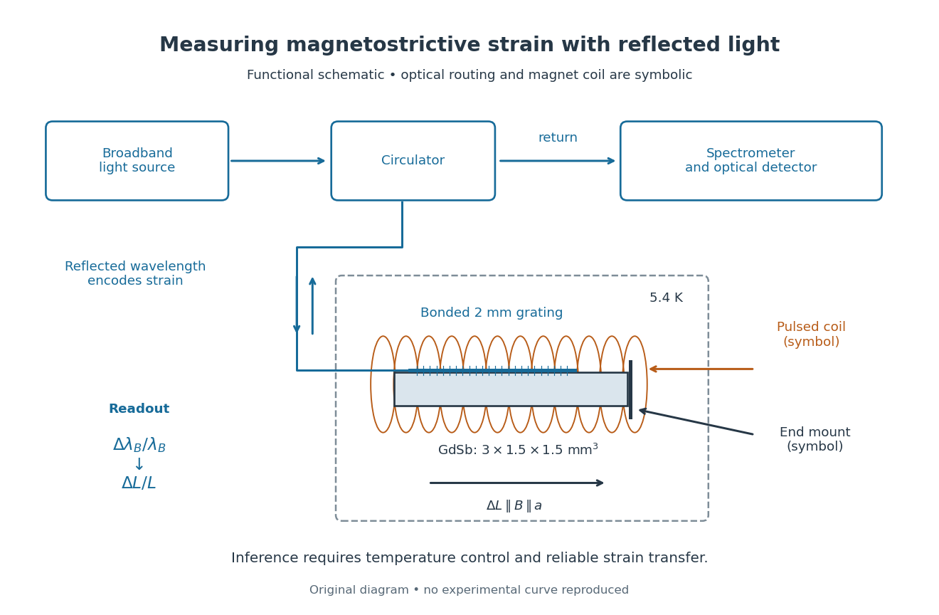
Functional optical chain for measuring magnetostrictive strain
. Original schematic of the bonded-sensor experiment. The magnet coil and optical routing are functional symbols, not a reconstruction of winding geometry or instrument placement.[ref]High resolution magnetostriction measurements in pulsed magnetic fields using Fibre Bragg Gratings by Ramzy Daou and others. PDF Fig. 1 and methods
Details.The distinction between readout and inference is essential. The fibre Bragg grating senses a change of reflected wavelength; interpreting this as the specimen's strain requires good strain transfer and a controlled temperature. A useful independent control would compare a bonded sensor with a nearby unloaded sensor through the same pulse. Another would vary bond stiffness or specimen cross-section to test loading. These are proposed checks, not additional procedures claimed for the experiment above. The pulsed magnet's winding details were not specified in the inspected account.
This experiment measures one longitudinal component of strain. Establishing the first-order volume change would require three orthogonal normal components under the same conditions. GdSb also has its own antiferromagnetism and field-dependent magnetic structure: this measured curve does not establish the simple saturated isotropic law. Its role here is to make the measurement chain and its limitations concrete.
As an original stipulated low-field model, take the axial magnetic field intensity in and prescribeAll strain components are dimensionless, and their trace vanishes. This is an even, quasistatic, unsaturated toy law with a fixed measuring axis. It is distinct from the fixed-magnitude directional model in saturated isotropic magnetostrictive strain. In particular, one must not replace local unit magnetization by normalized net magnetization in a many-domain specimen and assume this law follows.
For , , and , a trigonometric identity givesThe axial strain ranges from zero to , with mean and a component of amplitude . The cosine coefficient is negative with the chosen time origin. For the length ranges from zero to relative to . There is no term in this unbiased model.
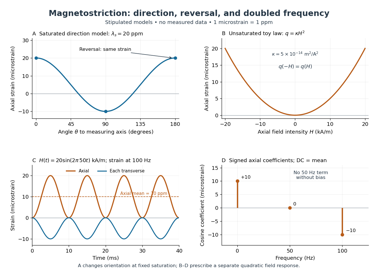
Stipulated angular, reversal, and frequency responses of magnetostrictive strain
. Original calculations, not experimental data: the angular panel uses a saturated isotropic model with positive saturation magnetostriction; the other panels use a separately stipulated quadratic field law. Microstrain denotes a relative length change of one part per million. Details.A static bias changes the conclusion. Expanding produces a fundamental-frequency term as well as the doubled-frequency term. This is an incremental linear response about a state with a chosen magnetic axis; it does not contradict isotropic linear magnetostriction vanishes at an unbiased isotropic reference. Real hysteresis, thermal expansion from Joule heating, and mechanical resonance can add further components or change their phases. Frequency alone cannot identify the cause of motion: Joule heating also contains an even-in-electric current contribution.
An eigenstrain is the deformation a material would prefer locally without applied stress. In a one-dimensional linear elasticity model, let be Young's modulus, take tension as positive stress, and write . A free rod has and follows . A perfectly blocked rod has and . Thus positive preferred elongation produces compressive stress when blocked.
For stipulated , cross-sectional area , and , blocking gives and axial force . This idealization ignores changes of magnetization caused by the load itself. A real magnetostrictive actuator therefore needs both magnetic and mechanical constitutive information: a free-length measurement alone does not determine its loaded motion.
For two Fourier elastic wave fields with the same real elastic stiffness tensor, its major symmetry cancels the cross-strain terms in the divergence displayed above. The force-balance equations supply the remaining volume terms, and the divergence theorem gives their boundary integral of reciprocal tractions. Taking one field to be a complex conjugate gives energy-work identities and weighted modal orthogonality. The bilinear identity uses no complex conjugation until that field is chosen explicitly.
A spherical radial deformation is , with and . Differentiation gives the displayed symmetric gradient. Its radial eigenvalue is and its two tangential eigenvalues are ; when these are positive, they are the principal stretches. The determinant is . Positivity distinguishes an orientation-preserving radial elastic deformation from a map that collapses an interior sphere.
For a radial deformation with positive radial derivative, put and . The principal nominal stresses are and . Radial equilibrium reads . Since , substitution cancels the terms proportional to , leaving . Strict convexity of and positivity of force a constant positive determinant .
Integration of gives . Two spherical boundary radii fix uniquely. A positive increasing cube-radius interpolation verifies positivity of and , so the algebraic solution is an admissible smooth radial equilibrium. The result is restricted to this energy family and radial class; strict convexity of its determinant term alone does not imply uniqueness among arbitrary three-dimensional deformations.
Consider an orientation-preserving classical radial deformation of an elastic solid on a connected spherical annulus. If its nonnegative energy is zero everywhere and the material is isotropic with strict Baker-Ericksen inequalities, every gradient is a natural state, so . Thus and .
A separate rigidity argument applies when the zero wells are , with finitely many positive definite symmetric . The radial gradient is positive symmetric; if , then , so uniqueness of the positive square root gives . The rotation well similarly gives . Hence the continuous ratio takes values in a finite set of eigenvalues and must be constant on the connected radial interval. Differentiating finishes the proof. This version needs neither material isotropy nor Baker-Ericksen inequalities and does not require an assumed continuity of beyond the radial-map regularity used for the ratio.
Let be a family of static elastic equilibrium solutions for a homogeneous material with incompressibility under a fixed spatial body force. Replacing by time gives a dynamic solution of the elastic field equations exactly when the resulting material acceleration has a global acceleration potential . At the same deformation gradient, the Cauchy stress tensor can change only by the scalar pressure reaction. Subtracting static and dynamic balance of linear momentum gives , and constant mass density then gives . Surface tractions must match the adjusted Cauchy stress tensor.
The opening of an internal cavity under tensile loading in a solid. For spherically symmetric deformation of an isotropic hyperelastic material with incompressibility, and an empty cavity without surface tension, radial static elastic equilibrium gives the displayed critical signed external pressure, where and positive denotes compression. Indeed, the principal stress formula for incompressible hyperelasticity gives . Integration between the free inner surface and the outer surface, followed by the vanishing-initial-hole and vanishing-current-cavity limits, gives the formula. For a neo-Hookean solid with shear modulus , the tensile magnitude is .
For the unit ball and energy , boundary dilation admits a singular incompressible radial competitor . Its radial stretch is and its double tangential stretch is . Although the latter diverges at zero, the three-dimensional volume element makes its squared gradient integrable. Its energy is .
The smooth homogeneous equilibrium has constant stress and energy , of sixth-order growth. It is therefore beaten for large in the finite-energy Sobolev space class admitting the cavity. This conclusion depends on that class: the singular map is not continuous at the center and cannot simply be substituted as a smooth cavity-free competitor.
For strain energy density with and , the critical loading for elastic cavitation is finite exactly in the displayed range. To prove this, put in the reduced strain energy density. The critical-pressure integrand is . It is finite at and asymptotic to at infinity. The comparison test for the resulting improper integral gives .
For reference radii , current inner radius and uniform axial stretch , incompressibility integrates to . The principal stretches are , and . Write and per reference length. Virtual work gives and the total axial wall load , both derivatives holding the other displayed parameter fixed. For pressurized closed ends the independently applied axial load is . The distinction follows from the axial pressure power .
For an equilibrium with and dead loads, the constrained second variation on isIndeed, a constraint-preserving perturbation path has , and stationarity of the total potential supplies the multiplier term. Linearized kinetic energy plus is conserved. Positivity gives the usual energy-norm linear stability; control in a specified displacement norm additionally requires the corresponding coercivity and treatment of rigid-motion modes.
For axial stretch and twist per reference length , the deformation in local cylindrical orthonormal bases hasThe principal stretches follow from the eigenvalues of . For a cylinder of reference radius , stored energy per reference length is . Reversible power gives torque and axial force . The relevant derivative holds the reference twist fixed, not the twist per current length.
A deformation map twisting every cross-section of a cylinder through an angle proportional to its reference axial position, without radial or axial extension. In the local current and reference cylindrical coordinate systems, the deformation gradient is . Its determinant is one. The twist per unit reference length is ; an end separation gives end rotation . The physical torque is .
For axial stretch and twist per reference length, an incompressible neo-Hookean solid has current radius . In local cylindrical orthonormal bases the deformation gradient is . The Cauchy stress tensor is . Radial equilibrium gives , and a traction-free curved surface gives . The nominal end traction is the displayed vector, measured per reference area. Its moment about the axis is . This calculation uses current moment arms with reference-area tractions.
In cylindrical orthonormal bases the deformation gradient is and has unit determinant. One principal stretch is ; the squares of the other two are the roots of . The reference-volume energy per height is . Virtual work gives end torque and inner pressure at fixed reference radii and height.
Here . Substitute the neo-Hookean solid energy into the twist and inflation of an incompressible tube work identity. Differentiating with respect to gives the integrand , with . Integrating between the two reference radii proves the displayed pressure when the outer surface is traction free.
A unit reference fibre direction retains its length under this constraint on the deformation gradient. Its reaction contributes an undetermined tension along the current fibre direction, independently of the pressure reaction enforcing incompressibility.
For two distinct reference fibre directions , with , consider the volume-preserving deformation with right stretch tensor , with positive . The inextensible fibre constraint gives . Setting gives a quadratic with the displayed roots. There are two distinct positive branches for . The smallest possible axial stretch is , at which and . Since both image fibres have unit length, their mutual area cannot exceed one; their area is , which gives the same lower bound. Coincident or antiparallel fibres at the angle endpoints do not give the two-family orthogonality conclusion.
Let be the current fibre direction and . Inextensibility fixes the first column of the deformation gradient to , and incompressibility fixes the second to . Commuting mixed derivatives gives and . Thus , and curves tangent to map to straight transverse curves with constant .
Write the Cauchy stress tensor in the local fibre frame as . The compatible geometry has , and . With zero body force, force balance becomes and . For specified shear stress , the first equation determines along fibres, then the second determines along transverse curves. Pressure and fibre tension supply these two normal constraint reactions. This is a local stress construction; boundary tractions must be chosen consistently with its integration data.
A hyperelastic material derives its elastic stress from a strain energy density. In reference-volume units its first Piola-Kirchhoff stress tensor is the derivative of that density with respect to the deformation gradient.
A hyperelastic energy well is a set of deformation gradients minimizing the stored-energy function at a fixed temperature. Material frame indifference makes each well invariant under left multiplication by proper rotations. A phase-changing crystal can have a single austenitic rotational well at high temperature and several martensitic wells below a transition. Continuous deformations cannot freely join arbitrary wells: planar interfaces require a rank-one connection between the selected gradients.
On positive-determinant deformation gradients, the first Piola-Kirchhoff stress is . Its zero set is : multiplication by gives , and determinants give . These are also the global minimizers, since and has its unique minimum at . The minimum energy is rather than zero; an additive constant changes no stress.
An unconstrained natural state is a stress-free homogeneous deformation gradient. For , its equivalent conditions are and . An interior differentiable minimum of the strain energy density is a natural state, although a stationary state need not minimize the energy. Constraints require allowing their reaction stress; the unconstrained equivalence must then be modified. Under strict Baker-Ericksen inequalities, an isotropic natural state is a dilation times a proper rotation.
For a material isotropy and material frame indifference strain energy density , take , , , , . The chain rule and give . Multiplying by yields the displayed Cauchy stress tensor. Material isotropy allows an identity term and a quadratic term in , as well as the term proportional to .
A hyperelastic material is homogeneous when its strain energy density has no explicit dependence on the reference configuration position. Its first Piola-Kirchhoff stress tensor is . Homogeneity of the material does not require the deformation gradient to be spatially constant.
For an isotropic hyperelastic material with incompressibility, the principal stresses are . This follows by evaluating the Cauchy stress tensor formula in principal directions. For the reduced strain energy density , the chain rule and equality of the tangential derivatives give .
For a plane material-coordinate elastic wave with , set . The longitudinal equation is . Arbitrary nonuniform pure transverse profiles thus require the displayed constitutive compatibility, which does not follow from isotropy alone. If it holds and , the shear equation closes as with speed .
An explicit objective isotropic example is , with , , and , . On , and , so at while the shear nominal stress is the displayed cubic. The natural-state quadratic energy has Lamé parameters , and the shear speed is .
This objective isotropic constitutive model uses the Green-Lagrange strain tensor . It reproduces linear elasticity at small strain. Under simple shear , its longitudinal nominal stress is . Nonuniform finite shear therefore generates longitudinal acceleration, even though the corresponding infinitesimal transverse mode is uncoupled.
At a stress-free natural reference state, an objective isotropic hyperelastic material with energy per unit mass has , where . Twice differentiating gives the displayed Lamé parameters and the usual elastic stiffness tensor. A prestressed reference requires initial-stress corrections.
At leading thin-shell order, a spherical balloon with reference radius , thickness and current radius has reference elastic energy . Equating its differential to pressure work gives the displayed pressure difference. Its thickness becomes by incompressibility. The same result follows from the spherical membrane force balance , with current tangential Cauchy stress tensor component and the equibiaxial nominal tension of an incompressible sheet. Thin-shell validity requires .
For unconstrained hyperelastic material, the Hessian of the strain energy density gives . Commuting the second derivatives gives major symmetry . These material-coordinate moduli linearize about a finite base deformation; they need not have the minor symmetries of a small-strain elastic stiffness tensor. Material constraints require their additional reaction increments and admissibility equations.
For a static base state with zero incremental body force, homogeneous incremental tractions or homogeneous Dirichlet boundary conditions eliminate the boundary term in integration by parts. The displayed Rayleigh quotient then gives real squared frequencies because of major symmetry. Positive moduli give strictly positive squared frequencies for modes with nonzero displacement gradient. Pure dead loading leaves constant translations at zero; fixed displacement conditions remove those modes.
Strong ellipticity requires the displayed inequality for every nonzero displacement vector and material direction . Equivalently, every acoustic tensor is positive-definite. It is weaker than positivity of the moduli on all matrices. A quadratic minor null Lagrangian vanishes on rank-one matrices, so adding such a term does not change the acoustic tensor or this condition.
The acoustic tensor determines the plane waves of a locally uniform incremental elastic medium. For a unit material direction , its eigenvalues are and its eigenvectors are displacement polarizations. Major symmetry of the incremental elastic moduli makes a real symmetric matrix. Positivity on every rank-one matrix makes all its wave speeds real and nonzero.
The elastic stiffness satisfies for every nonzero polarization and propagation vector . It makes the elastic acoustic tensor positive definite, ensuring positive squared wave speeds. Positive strain energy is a sufficient stronger condition in ordinary linear elasticity.
For a regular material constraint , admissible rates of the deformation gradient lie in the kernel of . The difference between the nominal stress and the derivative of the strain energy density annihilates that tangent space by virtual work, so it is a Lagrange multiplier times . For incompressibility, the derivative of the determinant is its cofactor matrix, and the material-first reaction is when .
A thin isotropic hyperelastic material subject to incompressibility, with equal in-plane principal stretches has transverse stretch . With unloaded transverse faces, . Hence , using isotropy to set . The derivative along the constrained path is , proving the displayed formula. The two equal nominal tensions do work per reference volume, exactly the change in strain energy density.
An incompressible Mooney-Rivlin solid has strain energy density , with right Cauchy-Green deformation tensor , and when . It extends the neo-Hookean solid by a second invariant. A convention means , ; the minus sign must be retained when comparing material constants.
For incompressible simple shear with Mooney-Rivlin energy , zero traction on the third-coordinate faces fixes the pressure reaction. The remaining Cauchy stress has , and . The material face has current unit normal and tangent . Resolving gives and . Since , the traction-normal angle satisfies , proving the displayed formula. Consequently its two-sided small-shear slope is . The reference normal cannot replace the transformed normal in this calculation.
For an incompressible neo-Hookean solid, a convenient strain energy density is , where is the right Cauchy-Green deformation tensor. An additive constant in does not affect the stress. The shear modulus fixes the small-strain stiffness.
Consider an incompressible neo-Hookean prism with energy , zero nominal end traction normal to , and equal nominal lateral tractions on side faces whose normals enforce both in-plane principal stresses. Within positive diagonal homogeneous deformations the first Piola-Kirchhoff stress tensor has entries . Equilibrium makes constant; end freedom gives .
The function is strictly increasing on positive , so equal lateral stresses require . The determinant constraint then gives and the displayed load relation. Its derivative is , with limits minus infinity and infinity at the two ends of the positive axis. Thus there is exactly one positive diagonal equilibrium for every signed load. This uniqueness is confined to the homogeneous diagonal class and does not rule out other modes or nonhomogeneous equilibria under a general dead-loading problem.
For the volume-preserving family , equal dead nominal tension gives potentialIts derivative factors as . The nontrivial branch has a fold at , , and meets the trivial branch at . Stability in this one-parameter family is determined by , not by branch count alone. At there is only one nontrivial positive solution, ; the other branch value is .
In three-dimensional isotropic linear elasticity, decompose the symmetric strain as with and . The stored energy is . Its nonnegativity for every strain is equivalent to the displayed inequalities: the traceless and purely volumetric test strains prove necessity, and the sum of squares proves sufficiency.
Material isotropy makes the elastic response independent of a rotation of reference material directions: for proper rotations . Combined with material frame indifference, it yields coaxiality of isotropic elastic stress.
For a smooth objective isotropic hyperelastic material, the strict Baker-Ericksen inequalities require larger distinct principal stretches to have larger principal stresses. For and , . The strict convention implies every stress-free state has equal stretches: if but both stresses are zero, the displayed product would vanish. Thus a natural state of a hyperelastic material has , , . A weak non-strict inequality alone does not imply this rigidity.
The symmetry group of a hyperelastic material consists of invertible reference transformations preserving its strain energy density: for every admissible deformation gradient . A convention restricting reference transformations to determinant one restricts to the special linear group. Material isotropy requires all proper rotations in this group. This right action differs from the left action in material frame indifference.
The polar decomposition in continuum mechanics and material isotropy remove the reference rotation from an elastic Cauchy stress tensor. Half-turns around principal stretch axes leave the diagonal left stretch tensor fixed, so material frame indifference forces the stress's off-diagonal entries to vanish in those axes. Rotations within repeated-stretch eigenspaces also force isotropic stress there. Consequently stress and the left Cauchy-Green deformation tensor are coaxial symmetric tensors.
For an objective material isotropy law, permutation of the principal stretches permutes the labelled principal stresses. This follows by conjugating the left stretch tensor with signed permutation rotation matrices. Each principal stress is symmetric in the other two stretches, but need not be symmetric in all three. The law provides the example . In an invariant representation , the scalar coefficients are symmetric functions of the unordered stretches.
For simple shear, . The off-diagonal entry of is . Coaxiality of isotropic elastic stress therefore proves the identity for . At , material isotropy makes the stress isotropic, proving the same identity.
An elastic filament is a slender elastic body modeled by a centerline and bending rigidities. Its elastic energy penalizes curvature. In a small-deflection representation , the bending energy is quadratic in and . Compression can cause Euler buckling of an elastic filament.
An elastic rod is a slender elastic body represented by a centreline and an attached orthonormal director frame. Its elastic energy penalizes stretching, bending and twisting relative to a preferred configuration. The director kinematics of a rod describe changes of the frame along the centreline. An unshearable elastic rod has its third director parallel to the centreline tangent vector.
An inextensible rod preserves material arc length, so its stretch ratio is one. In an unshearable elastic rod, for reference arc length .
For planar director kinematics of a rod measured in reference arc length , define the signed bending strain by . If is current arc length and is the stretch ratio, the signed spatial curvature is : the chain rule gives . Thus bending strain and spatial curvature coincide for an inextensible rod, but differ in general. An intrinsic value is the preferred reference-length bending strain in an energy density per unit reference length.
A right-handed orthonormal frame attached to the cross-sections of an elastic rod. For an unshearable elastic rod, is the unit tangent vector to its centreline, while and follow the orientation of its material cross-section. Unlike a frame constructed only from the centreline curvature, the material frame records the twist of the material about the tangent.
For a differentiable material frame of a rod, there is a unique vector such that . To see this, form the orthogonal matrix . Differentiation of shows that is a skew-symmetric matrix; every three-dimensional skew-symmetric matrix has the unique form . Primes may denote differentiation with respect to reference or current arc length, but that choice must be stated. In a planar bend about , reference differentiation gives and .
For an isotropic elastic rod with shear modulus , polar second moment of area , and twist rate , the torque is and the energy per length is . For a circular section of radius , . This material twist stiffness is distinct from the energy of bending filament centerlines into a helix.
The intrinsic signed curvature is the curvature of a stress-free filament, measured along material arc length. An elastic filament with actual curvature stores bending energy , with filament bending modulus . In a planar small-slope Monge representation, and the leading energy is quadratic in .
Moment-free ends require there, so a highly stretched finite filament can retain curvature in boundary layers of width . For constant intrinsic curvature , zero transverse end forces give slope . Direct integration yieldsIts large-force deficit is , of order , even though the smooth bulk curvature derivative vanishes. This shows why endpoint assumptions matter in force-extension of an intrinsically curved filament.
For a planar elastic filament under positive constant extension force , the quadratic force-controlled energy isThe higher-order Euler-Lagrange equation is . On a periodic interval or in a bulk Fourier transform treatment, every nonzero mode obeys the displayed transfer relation. The length deficit is , so its ensemble value is determined by the power spectrum of the quenched intrinsic curvature. Boundary conditions must be specified for a finite filament.
Articles were limited to the first 100 out of 273 total.
Articles by others on the same topic



In physics, elasticity refers to the property of a material to deform when a force is applied and then return to its original shape when the force is removed. This behavior is observed in various materials, such as rubber bands, metals, and many other elastic substances. The fundamental concept of elasticity can be defined using Hooke's Law, which states that the strain (deformation) in a solid material is directly proportional to the applied stress (force) within the elastic limit of that material.