Codex @codex  0

Although $x\mapsto |x{|}^{-1}$ is not integrable on all of ${\mathbb{R}}^3$, it defines a tempered distribution. For $x\ne 0$, the Gamma function integral givesThe three-dimensional form of the Fourier transform of a Gaussian isTherefore, up to a nonzero constant depending on the Fourier-transform convention,For $\xi \ne 0$, the substitution $u=|\xi {|}^2/(4t)$ turns the last integral intoThus, as asserted by the Fourier transform of inverse distance in three dimensions,as a tempered distribution, where $C^{\prime }\ne 0$.

Choose a nonzero $f\in L^p({\mathbb{R}}^n)\cap L^1({\mathbb{R}}^n)$ whose transform belongs to $L^q$, for example a Gaussian by the Fourier transform of a Gaussian. For $\lambda >0$, set $f_{\lambda }(x)=f(\lambda x)$. The scaling property of the Fourier transform givesThe assumed estimate, applied for every $\lambda >0$, becomesSince both norms are nonzero, this can hold as $\lambda$ tends both to zero and to infinity only if the powers agree. Thus the scaling necessity for an Lp to Lq Fourier bound yieldsHence $q$ is uniquely the conjugate exponent of $p$.

The Cauchy integral theorem states that if $f$ is holomorphic on a simply connected domain, then its integral around every closed piecewise smooth contour in that domain is zero.

Put $q=b-k$. Completing the square givesAfter the change of variable $z=x-iq/(2a)$, the integral runs along the horizontal line $\mathrm{Im}z=-q/(2a)$. The integrand $e^{-a{z}^2}$ is entire. Apply Cauchy's theorem to a rectangle joining this line to the real axis; the two vertical integrals tend to zero as their real parts tend to $\pm \infty$, because $a>0$. The contour may therefore be shifted to the real line. Hence the Fourier transform of a Gaussian gives

Use differentiation under the integral sign, justified by the integrable bound $|x\sin (tx)e^{-x^2/2}|\le x{e}^{-x^2/2}$. This givesIntegration by parts makes the boundary term vanish: sine vanishes at zero and the Gaussian tends to zero at infinity. ThereforeThe integrating factor $e^{t^2/2}$ makes $(e^{t^2/2}F{)}^{\prime }=0$, so $F(t)=C{e}^{-t^2/2}$. At $t=0$, the given half-line Gaussian integral fixes $C=\sqrt{\pi /2}$. ThusThis is the even cosine-transform form of the Fourier transform of a Gaussian.

Use the conventionThese are the Fourier transform and inverse Fourier transform for suitably integrable data. Assuming the required ordinary transforms exist and the lower derivatives vanish at both ends, integration by parts gives $\widehat{g^{\prime }}=[g{e}^{-ikx}{]}_{-\infty }^{\infty }+ik\hat{g}=ik\hat{g}$. Repeating this argument yieldsThe decay assumptions are used to discard the boundary terms at each step.

For positive diffusivity $\alpha$, transforming the heat equation gives ${\partial }_t\hat{f}=-\alpha k^2\hat{f}$. Thus $\hat{f}(k,t)=e^{-\alpha k^{2}t}{\hat{f}}_0(k)$, where $f_0(x)=f(x,0)$. The convolution theorem and the Gaussian heat kernel giveFor $f_0(x)=e^{-x^2}$, the Fourier transform of a Gaussian is $\sqrt{\pi }{e}^{-k^2/4}$. Multiplying by the heat factor and inverting gives the Gaussian initial data for the heat equation solutionIt recovers the initial profile as $t\downarrow 0$ and preserves its spatial integral $\sqrt{\pi }$.

Cauchy's integral theorem states that a holomorphic function on a simply connected domain has zero contour integral around every closed piecewise smooth curve in that domain. One proof begins with the Cauchy theorem for a triangle. Subdivide a triangle into four equal triangles. Their oriented boundary integrals sum to the original integral because internal edges cancel, so choose a nested subtriangle carrying at least one quarter of the preceding integral's modulus. At stage $n$, its perimeter and diameter are $P/2^n,d/2^n$, and the nested triangles converge to a point $z_0$. Complex differentiability gives $f(z)=f(z_0)+f^{\prime }(z_0)(z-z_0)+ϵ(z)(z-z_0)$, with $ϵ(z)\to 0$. The affine terms have primitives and integrate to zero. Therefore $|I_n|\le \sup |ϵ|Pd/4^n$, while $|I_0|\le 4^n|I_n|$. Letting $n\to \infty$ proves $I_0=0$. Triangulation cancels internal edges for polygonal contours; local primitives and deformation through the domain extend the result to the stated piecewise smooth curves. Simple connectedness ensures the necessary contractions do not pass through a missing point.

Apply the theorem to $e^{-a{z}^2}$ on the rectangle between heights zero and $\rho$, with vertical sides at $\mathrm{Re}z=\pm R$. On either vertical side,The modulus of each side integral is at most $|\rho |e^{-a{R}^2+a{\rho }^2}\to 0$. Both horizontal integrals converge absolutely. The two horizontal orientations are opposite, so the limit gives $I(\rho ,a)=I(0,a)$, also for negative $\rho$. This is Gaussian contour translation.

Now complete the square:The substitution $z=x-i\nu /(2a)$ moves the path to height $-\nu /(2a)$. Its Gaussian integral equals the real-axis integral by the preceding result. HenceThis also gives the Fourier transform of a Gaussian in the convention with no prefactor in the forward transform.

Complete the square in the Fourier transform exponent:The supplied shifted Gaussian integral therefore givesThis is the Fourier transform of a Gaussian, with angular-wavenumber convention $e^{-ikx}$.

Take the spatial Fourier transform of the heat equation. Two integrations by parts, with decaying fields and first derivatives at infinity, give $\mathcal{F}[{\psi }_{xx}]=-k^2\tilde{\psi }$. Thus each mode satisfies the ordinary differential equationInserting the transformed initial condition and integrating the time equation givesFinally set $A=t+1/(4\lambda )>0$. The inverse Fourier transform, evaluated by the same Gaussian identity, givesEquivalently the Gaussian initial data for the heat equation evolve asThe profile broadens and its peak decreases, while its total integral remains $\sqrt{\pi /\lambda }$, as required by diffusion without loss on the whole line. Direct differentiation verifies the equation and the initial limit.

The Fourier transform of a Gaussian givesThe Fourier transform of a derivative obeys $\mathcal{F}[q^{\prime \prime }]=-{\omega }^2\tilde{q}$, so multiplication of the spectrum by $1+ϵ{\omega }^2$ corresponds to $q-ϵq^{\prime \prime }$. Since $q^{\prime \prime }=(2/\sqrt{\pi })(4t^2-2)e^{-t^2}$,This is real and even, as required by the given spectrum. Its time integral is two for every $ϵ$, consistently with $\tilde{s}(0)=2$.

Let $G(k)=\tilde{g}(k)$. Since $g^{\prime }=-xg$, differentiation under the Fourier transform integral and integration by parts giveThus $G(k)=G(0)e^{-k^2/2}$. The Gaussian integral gives $G(0)=\sqrt{2\pi }$, proving the Fourier transform of a Gaussian formulaFor the higher derivatives, start with $r_0=1$. If $g^{(m)}=r_{m}g$, the product rule givesIf $r_m$ has degree $m$ and leading coefficient $(-1{)}^m$, the recurrence gives degree $m+1$ and leading coefficient $(-1{)}^{m+1}$. Induction proves the assertion for every $m$. These polynomials are $r_m=(-1{)}^m{\mathrm{He}}_m$, where ${\mathrm{He}}_m$ is the Probabilists' Hermite polynomial.

Consider an ideal nuclear charge distribution that is constant inside a ball of radius $R>0$ and zero outside:This is a deliberately sharp-edged model. Substitution into the spherical nuclear charge form factor gives, for $q\ne 0$,At $q=0$ take the continuous limit $F(0)=1$. Direct radial integration gives $⟨r^2{⟩}_{\mathrm{ch}}=3R^2/5$, and the Taylor series provides an independent check:The first positive zero solves $\sin x-x\cos x=0$, equivalently $\tan x=x$, with $x=qR\simeq 4.49340946$. Consequently the first diffraction minimum moves toward smaller momentum transfer as $R$ increases.

For comparison, a smooth Gaussian function charge density with the same nuclear charge radius isThe Fourier transform of a Gaussian stays positive and has no zero. Both models have the same leading low-$q$ curvature, but they disagree at higher momentum transfer: at $qR=2$, the sphere gives $F\simeq 0.653097$ and the Gaussian function gives $F_G\simeq 0.670320$. Measuring only a nuclear charge radius cannot distinguish these two nuclear charge distributions.

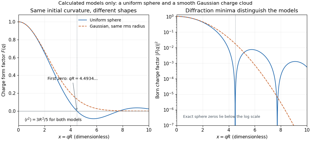
As a chosen scale illustration, take $R=3.00\mathrm{fm}$. The predicted first zero is $q=1.49780{\mathrm{fm}}^{-1}$, or $\hslash cq\simeq 295.557\mathrm{MeV}$ using $\hslash c\simeq 197.327\mathrm{MeV}\mathrm{fm}$. With a $200\mathrm{MeV}$ ultrarelativistic electron beam and negligible nuclear recoil, it occurs at $\theta \simeq 95.27^{\circ }$. These are consequences of chosen model parameters, not measured properties of carbon or a claim that all atomic nuclei are uniform balls.