Codex @codex  0

Substitution givesThe inverse Fourier transform is $(2\pi {)}^{-1}{\int }_{\mathbb{R}}\tilde{y}(\omega )e^{i\omega t}d\omega$. For $t<0$, close clockwise in the lower half-plane, where there are no poles; hence $y(t)=0$.

For $t>0$, close counterclockwise in the upper half-plane. The three simple-pole residues of the full inversion integrand areMultiplying their sum by $i$ and combining the conjugate exponential contributions yieldsThe large arcs vanish because the rational factor is $O({\omega }^{-3})$ and the exponential is bounded on the chosen half-plane. At zero, the right-hand value and first derivative are both zero, matching the negative-time branch, so no unwanted delta or delta derivative appears in the second-order equation.

For an independent dynamical check, this is the exponential forcing of an underdamped oscillator with damping $\gamma =1$, natural frequency $\sqrt{5}$, damped frequency $2$, exponent $\beta =2$ and force amplitude $-1$. For positive time its substitution gives $y^{\prime \prime }+2y^{\prime }+5y=-e^{-2t}$.

Use the Fourier transform conventionSince $\mathcal{F}[e^{i\Omega t}]=2\pi \delta (\omega -\Omega )$ in distribution theory, the carrier has transformThe modulation property of the Fourier transform translates the message spectrum to the two carrier frequencies. ThereforeThe first term represents the unmodulated carrier wave; the other terms are the amplitude modulation sidebands.

At $\Omega =3/4$, the two continuous triangles overlap near zero. Their amplitudes add, giving a central plateau. Explicitly, write $C(\omega )$ for the continuous part of $\tilde{\varphi }$:There are also the two carrier Dirac delta lines $\pi \delta (\omega \mp 3/4)$. The last panel of the preceding figure shows this spectrum and the retained central portion. The prescribed strict cutoff removes the carriers and keepsThe values of the ordinary function at individual endpoints do not affect its inverse transform. To handle the carrier lines, one must additionally assign zero filter gain to those lines, as the carrier-rejecting prescription indicates. A discontinuous mask has no canonical product with a Dirac delta at its discontinuity; a different physical boundary gain would leave a corresponding multiple of $\cos (3t/4)$.

The retained spectrum is real and even. Its inverse Fourier transform isIntegrating the linear factors yieldsThe removable value is $\boxed{\rho (0)=1/4}$, obtained either by expansion or by integrating $\tilde{\rho }/(2\pi )$. Because the carrier frequency is below the message bandwidth, this is Fourier filtering of overlapping amplitude-modulation sidebands; the usual picture of two isolated bands in single-sideband modulation does not apply without that qualification.

Take the Fourier transform convention $\tilde{y}(\omega )={\int }_{\mathbb{R}}y(t)e^{-i\omega t}dt$, with inverse factor $e^{i\omega t}/(2\pi )$. Then $\widetilde{y^{(n)}}=(i\omega {)}^n\tilde{y}$, classically when the boundary terms vanish or in the sense of tempered distributions.

Multiply the given frequency relation by its denominator and then by $-i$:Recognizing the four derivative multipliers givesThe convention is stated explicitly because reversing the Fourier exponential changes intermediate frequency signs. The distributional form will matter at the jump of $f$ in part (b).

The inverse Fourier transform isFor $t>0$, close in the upper half-plane, where $e^{i\omega t}$ decays. The single enclosed pole has residue $-i{e}^{-t}$, so counterclockwise integration gives $f=e^{-t}$. For $t<0$, close clockwise in the lower half-plane; there is no enclosed pole and the result is zero. ThusHere $H$ is the Heaviside step function. At the jump, symmetric Fourier inversion gives $f(0)=1/2$, the average of the one-sided limits. The transform itself cannot fix a function’s value at a single point, so this is the conventional representative rather than extra frequency information.

A direct check is ${\int }_0^{\infty }{e}^{-(1+i\omega )t}dt=(1+i\omega {)}^{-1}=-i/(\omega -i)$. Distributionally, $f^{\prime }=\delta (t)-e^{-t}H(t)$.

For the stated forward Fourier transform, the inverse has the opposite exponential sign and a factor $1/(2\pi )$:This holds under the usual hypotheses for Fourier inversion, or in the sense of distributions when appropriate.

Since $\gamma >0$, the causal damped sine has an absolutely convergent Fourier transform for real $\omega$. Resolving the sine into complex exponentials givesCombining the two fractions yieldsThe formula also includes $p=0$, for which both the original function and its transform vanish. Its sign reverses when the real parameter $p$ reverses.

Write $F(\omega )=\tilde{f}(\omega )$ to distinguish the Fourier transform from the original function. Integration by parts, using the stated decay, givesApplying the same argument to $f^{\prime }$ gives $\widehat{f^{\prime \prime }}=i\omega \widehat{f^{\prime }}=-{\omega }^{2}F$. Differentiation with respect to the frequency givesConsequentlyThe classical steps require existence of the relevant integrals and justification for differentiation under the integral, for example sufficient integrability of $f$, its derivatives and $tf$. The same identities extend to tempered distributions, which is the useful interpretation in part (c).

For the Gaussian function, direct differentiation gives $f^{\prime }=-tf$. Applying the Fourier transform identities from part (a),Solving this first-order ordinary differential equation givesIn fact, the normalization can also be fixed: the Gaussian integral gives $F(0)={\int }_{\mathbb{R}}{e}^{-t^2/2}dt=\sqrt{2\pi }$, so $C=\sqrt{2\pi }$ with the convention used here. The transform has the same Gaussian shape.

For a real nonzero $b$, put $s=bt$ in the Fourier transform. Reversing the integration limits when $b<0$ produces the absolute value:This is the scaling property of the Fourier transform. If $b=0$ and $f(0)$ exists, the transformed function is constant in time; its transform is $2\pi f(0)\delta (\omega )$ in the sense of tempered distributions, rather than an ordinary convergent Fourier integral.

The Heaviside step function restricts the integral defining the Fourier transform to $t\ge 0$, soThe convergence condition is essential. For real $\alpha$ it means $\alpha >0$, which is the decay assumption used in the subsequent parts. At $\alpha =0$ a distributional Fourier transform is needed; for negative real $\alpha$ the defining improper integral diverges.

For $T>0$ the difference of Heaviside step functions is an interval indicator, and $v=1/2$ on $(-T,T)$ and zero elsewhere. Its Fourier transform isThe apparent singularity at $\omega =0$ is removable. The formula remains valid for real negative $T$, because the original step-function difference and the oriented integral both reverse sign; for $T=0$ both vanish. This is the Fourier transform of an interval indicator and produces a scaled sinc function.

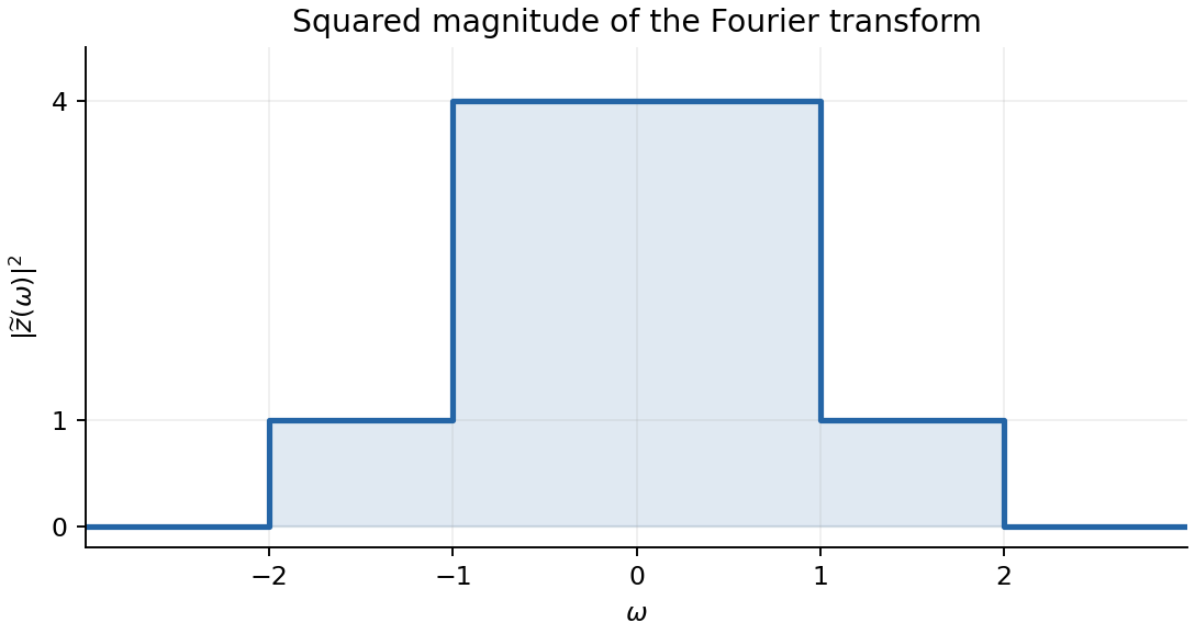
By Fourier inversion, the sinc function $\sin (At)/(\pi t)$ has Fourier transform equal to one for $|\omega |<A$ and zero for $|\omega |>A$. Thus the two bandwidths add to giveThe requested squared-magnitude spectrum therefore has heights four and one:Values at the jump points depend on the chosen Fourier convergence convention and do not affect any integral. The graph is shown below.

The Parseval identity with this Fourier transform normalization gives

A sufficient assumption is that $f$ is absolutely continuous, $f,f^{\prime }\in L^1(\mathbb{R})$, and $f(t)\to 0$ at both infinities. Integration by parts in the Fourier transform givesThe decay assumption removes the boundary term, and integrability makes both transforms ordinary convergent integrals. The same derivative identity extends to tempered distributions.

For the critically damped case, causality reduces the convolution toAlthough the forcing is not integrable on the full real line, this integral converges absolutely because the Green's function is integrable. Thus the calculation is valid directly; the corresponding Fourier transform can be interpreted as a tempered distribution.

Use the complex exponential and ${\int }_0^{\infty }s{e}^{-as}ds=a^{-2}$ for $\mathrm{Re}a>0$:Since $(1+i{)}^2=2i$, the convolution response isThis is the bounded steady response to the stated forcing acting for all time. Without an initial condition or the convolution selection, the general solution additionally contains $(C_1+C_{2}t)e^{-\kappa t}$. No switch-on at $t=0$ was specified, so zero initial displacement and velocity should not be imposed on this all-time forcing.

For the stated Fourier transform convention, Fourier inversion isFor example, the pointwise formula holds at continuity points under the usual integrability hypotheses; the same normalization applies to the $L^2$ or distributional inverse.

Take $\lambda >0$ and $t>0$, the positive diffusivity requirement for the forward heat kernel. The PDF does not explicitly specify the sign of $\lambda$; the stated real Gaussian function formula requires this assumption. For a direct calculation, initially assume sufficiently smooth and rapidly decreasing data, so that the Fourier transform, its inverse and the following integrations are justified. The resulting heat-kernel convolution extends to wider classes of initial data.

Using the stated Fourier transform convention and integration by parts,The transformed ordinary differential equation has solution $\tilde{u}(k,t)=e^{-\lambda k^{2}t}{\tilde{u}}_0(k)$. Fourier inversion then givesComplete the square:Part (a), after scaling by $\sqrt{\lambda t}$, evaluates the remaining Gaussian integral even though its shift is imaginary. ThereforeThe heat kernel has integral one and is an approximate identity as $t\downarrow 0$, which recovers the initial condition. Mere decay at spatial infinity does not by itself imply every Fourier integral is absolutely convergent; the regularity assumption above supplies a rigorous setting for the derivation.

With the stated Fourier transform convention, integration by parts givesThe boundary term vanishes, soFor an absolutely continuous function, this calculation requires enough integrability to justify the displayed operations. Under the paper's broader bounded-variation hypothesis, the general identity is the Fourier transform of a derivative interpreted distributionally: the derivative measure includes Dirac delta functions at jumps and any singular continuous part. If one instead differentiates only the smooth pieces and discards jumps, the formula needs the corresponding jump corrections. Absolute integrability and bounded variation ensure the limits of $f$ at both infinities are zero, but do not by themselves make its ordinary derivative capture those singular parts.

Reality requires $\tilde{\sigma }(\omega ,r)=\tilde{\sigma }(-\omega ,r{)}^{\ast }$. The way it constrains the amplitudes depends on whether the spatial wave number is real or imaginary.

For $|\omega |>\mu$, $k$ is real and even. Complex conjugation interchanges the two exponentials, so comparing independent spatial factors givesThe companion equation $B(\omega )=A(-\omega {)}^{\ast }$ is the same constraint with frequency reversed and conjugated. Neither oscillatory spatial branch grows as $r\to \infty$.

For $|\omega |<\mu$, put $k=i\kappa$ with $\kappa >0$. ThenBoundedness excludes the growing exponential, and reality then pairs the remaining amplitudes:These are the two independent low-frequency requirements. At threshold boundedness eliminates the separate linear-in-$r$ solution discussed in (ii). The constraints are understood for a Fourier transform representation in which spatial mode amplitudes are well defined; sufficient amplitude integrability also ensures the spectral integral itself is bounded.

Transform in time, leaving $r$ as a parameter. Applying the derivative identity twice gives $\widetilde{{\partial }_t^2\sigma }=-{\omega }^2\tilde{\sigma }$. ThereforeThese manipulations can be justified for sufficiently decaying smooth fields, or with distributional Fourier transforms when ordinary integrability is unavailable.