Codex @codex  0

Use the trigonometric identity $2{\cos }^2(ax)=1+\cos (2ax)$ and express the cosine as a sum of two complex exponentials. The Fourier transform of each exponential is a shifted Dirac delta distribution:By linearity,The original function does not decay and is not absolutely integrable on the real line, so this answer is a tempered distribution, rather than an ordinary convergent Fourier integral. Its three lines represent the constant part and the two opposite spatial frequencies.

The input is even, so its Fourier transform is real and even. Decomposing the cosine into complex exponentials and integrating over its support givesCombining the fractions and using the angle addition formula yieldsThe apparent poles at $k=\pm 1$ are removable singularities; either the integral or the sine-quotient limit gives $\tilde{f}(\pm 1)=a+\sin (2a)/2$.

If $\cos a\ne 0$, expansion of the denominator givesThe oscillatory envelope is therefore $O(|k{|}^{-1})$. At $a=\pi /2+n\pi$, $n=0,1,2,\dots$, the endpoint values vanish and the first term cancels:This gives an $O(|k{|}^{-2})$ envelope. At general $a$ the truncation creates jumps in the function; at these special values it leaves the function continuous but creates jumps in its first derivative. Each additional degree of endpoint smoothness gives another inverse power, as explained by Fourier decay from a derivative jump. The exact example is the Fourier transform of a truncated cosine; isolated zeros of its oscillatory factors do not change the envelope order.

With the stated Fourier transform convention, the exponential transform is a shifted Dirac delta distribution:Writing the sine as $(e^{i{\omega }_{0}t}-e^{-i{\omega }_{0}t})/(2i)$ then givesThese are tempered distributions, since the time-domain functions are not integrable on the full real line. The second formula also correctly vanishes when ${\omega }_0=0$.

For integrable functions $f,g$, Fubini's theorem justifies exchanging the two integrals in the Fourier transform of the convolution. Set $s=x-t$ to obtainThis proves the convolution theorem with the stated normalization:

Direct evaluation gives the first Fourier transform:For the even triangular function, the odd sine part integrates to zero. Two elementary integrations by parts or one evaluation of the cosine integral giveThe values at zero are the respective areas, agreeing with the removable limits. Therefore $\tilde{g}={\tilde{f}}^2$. By the convolution theorem and uniqueness of the Fourier transform,There is also a direct interpretation: the convolution is the length of overlap of the intervals $(-1/2,1/2)$ and $(x-1/2,x+1/2)$, giving exactly that triangular profile.

The Parseval identity for this Fourier transform convention isApply it to $h=g$. Its squared norm is $2{\int }_0^1(1-x{)}^{2}dx=2/3$, soUnder $k=2x$, the last integrand times $dk$ becomes $2{\sin }^{4}xdx/x^4$. ConsequentlyThe integrand has continuous value $1$ at zero and decays integrably at infinity, so this is an ordinary convergent improper integral.

Use the Fourier transform convention $\tilde{h}(k)={\int }_{\mathbb{R}}{e}^{-ikx}h(x)dx$. Split at zero and integrate the decaying exponentials:The transform is real and even because $h(x)=e^{-|x|/L}$ is real and even.

Let $G(k)=\tilde{g}(k)$. Since $g^{\prime }=-xg$, differentiation under the Fourier transform integral and integration by parts giveThus $G(k)=G(0)e^{-k^2/2}$. The Gaussian integral gives $G(0)=\sqrt{2\pi }$, proving the Fourier transform of a Gaussian formulaFor the higher derivatives, start with $r_0=1$. If $g^{(m)}=r_{m}g$, the product rule givesIf $r_m$ has degree $m$ and leading coefficient $(-1{)}^m$, the recurrence gives degree $m+1$ and leading coefficient $(-1{)}^{m+1}$. Induction proves the assertion for every $m$. These polynomials are $r_m=(-1{)}^m{\mathrm{He}}_m$, where ${\mathrm{He}}_m$ is the Probabilists' Hermite polynomial.

By the two Fourier transform rules in part (b),Consequently transforming the differential equation givesorThe inverse Fourier transform gives the reverse implication under the same regularity hypotheses. This expresses the Fourier symmetry of the quantum harmonic oscillator operator.

Part (b) shows that the transform of $g_n$ is $q_n(k)e^{-k^2/2}$ with $q_n$ of degree $n$. Part (c) shows that it solves the same eigenvalue equation as $g_n$, with the same ${\mu }_n$. The assumed uniqueness of the polynomial solution of each degree therefore forces $q_n=c_n{p}_n$; hence ${\tilde{g}}_n=c_n{g}_n$.

The constants can also be determined. Substituting $g_n=p_n{e}^{-x^2/2}$ into the equation gives the Hermite differential equationComparison of the leading coefficient yields ${\mu }_n=-(2n+1)$. If the leading coefficient of $p_n$ is $a_n$, part (b) gives leading coefficient $\sqrt{2\pi }(-i{)}^n{a}_n$ for $q_n$. ThusThus Hermite functions are Fourier eigenfunctions with the paper's unnormalized Fourier transform; dividing that transform by $\sqrt{2\pi }$ gives the unitary eigenvalues $(-i{)}^n$.

The signal is continuous at zero with $f(0)=1$. Its envelope is $e^{-\lambda |t|}$, but its angular frequency falls from $2$ on the incoming side to $1$ on the outgoing side. Its one-sided slopes are $f^{\prime }(0^{-})=\lambda$ and $f^{\prime }(0^{+})=-\lambda$, producing a cusp at the peak. Both tails decay to zero.

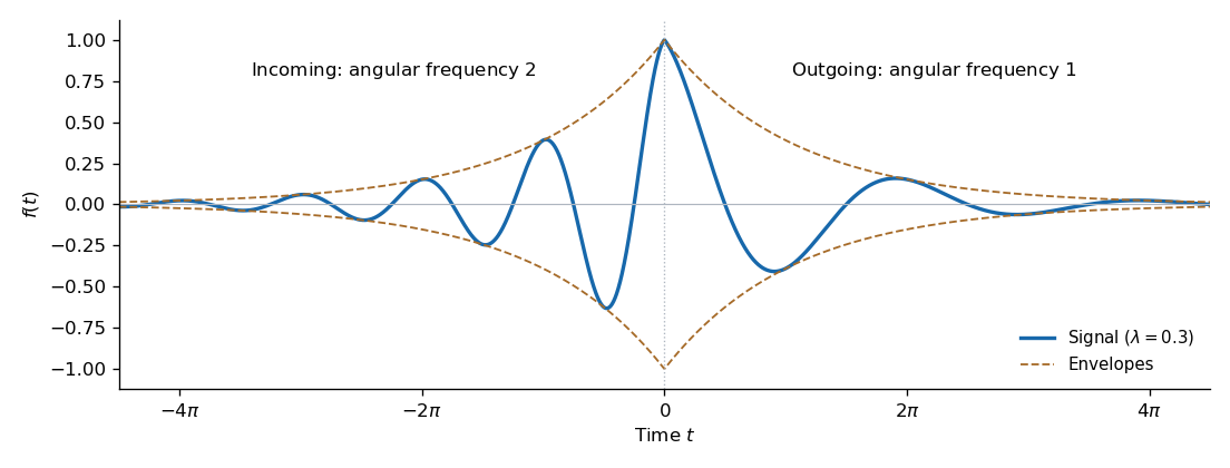
Use $\tilde{f}(\omega )={\int }_{\mathbb{R}}{e}^{-i\omega t}f(t)dt$. Expanding each cosine into two exponentials and integrating its half-line givesEquivalently,The positive $\lambda$ guarantees convergence of the Fourier transform integrals.

With the paper's Fourier transform convention, the Fourier inversion theorem givesThis holds at continuity points under the usual inversion hypotheses; at a jump with one-sided limits it gives their mean. The factor $1/(2\pi )$ and the sign change in the exponential are part of this normalization.

Insert the inverse Fourier transforms of $f$ and its complex conjugate, initially under enough decay to justify interchanging integrals:The middle step uses the stated Dirac delta distribution identity, and the last uses its sampling property. This is the Parseval identity for the chosen normalization. Approximation extends the result to square-integrable functions, including the function used below.

The real odd function has a purely imaginary odd Fourier transform. Setting $A=\pi /2$ and using a product-to-sum identity,The apparent singularities are removable. Direct evaluation or limits giveIn particular, the transform stays finite where its numerator and denominator both vanish.

Use the Fourier transform conventionThe convolution is $(f\ast g)(t)={\int }_{-\infty }^{\infty }f(\tau )g(t-\tau )d\tau$. For integrable $f,g$, Fubini's theorem and the substitution $s=t-\tau$ giveHence the convolution theorem is

Take the causal solution, extending the input and output by zero before the device starts at $t=0$. The two zero initial conditions ensure that this extension adds no impulsive terms to the first two distributional derivatives. The Fourier transform of a derivative is multiplication by $i\omega$, soFactoring the quadratic and taking partial fraction decomposition yieldsThe inverse Fourier transform follows directly by integrating decaying exponentials:where $H$ is the Heaviside step function. This damped-oscillator impulse response has $R(0^{+})=0$ and $R^{\prime }(0^{+})=1$, as required for a unit impulse.

Use the same Fourier transform convention, now in the sense of tempered distributions, since the homogeneous oscillations are not integrable. Transforming givesSince $q>0$, the two roots are distinct. A distribution annihilated by this polynomial is a linear combination of Dirac delta distributions at its roots:Fourier inversion therefore givesThe constants may be complex. Differentiating the factor $e^{-irt}$ also verifies that the original ordinary differential equation reduces to $\ddot{\psi }+q^2\psi =0$ for $\varphi =e^{-irt}\psi$.

Assume first that $f$ and $g$ are integrable functions, so that Fubini's theorem justifies changing the order of the two integrals. In the defining Fourier transform of the convolution, put $y=x-x^{\prime }$:This proves the convolution theorem with the stated normalization:

Direct evaluation of the Fourier transform gives, for $k\ne 0$,At $k=0$ the defining integral is the interval length, so $\boxed{\tilde{g}(0)=2}$. This also equals the continuous limit of the displayed formula.

The convolution $(g\ast g)(x)$ is the length of the overlap of $(-1,1)$ with $(x-1,x+1)$. This overlap has length $2-|x|$ when $|x|<2$ and zero otherwise, so $u=g\ast g$. The convolution theorem now givesThe value at zero is also the area of the triangular function, providing a normalization check on its Fourier transform.