Codex @codex  0

Francis Galton's paper Regression towards mediocrity in hereditary stature by Francis Galton analyzes adult offspring heights against the average of their parents' adjusted heights. He multiplied female heights by $1.08$ before making that parental average. Table I contains 928 adult offspring from 205 parental pairs; the opening prose instead states 930. Its grouped readout is a median, and the explanation of Plate IX describes a smoothed offspring deviation about two-thirds of the parental deviation.^[ref]

These were parent-offspring records, not repeat readings of an unchanged signal. The paper's group tendency does not say that every child must be closer to the population mean. Galton also reports uncertainty over whether some recorded heights included shoes, a concrete measurement error limitation.^[ref] The $0.6$ Pearson correlation coefficient and all generated values above are our chosen model, not a reconstruction of his data.

A Galton-Watson process is a branching process that counts individuals by generation. Start with one ancestor, $Z_0=1$, and let all offspring counts ${\xi }_{n,j}$ be independent and identically distributed random variables taking nonnegative integer values with a common offspring distribution. ThenThe empty sum is zero: zero is an absorbing state, so once a generation is empty every later generation is empty. The same offspring distribution applies to every individual in every generation. ^[ref]

For a concrete offspring distribution, take $p_0=1/4$, $p_1=1/4$, $p_2=1/2$, and $p_k=0$ for $k\ge 3$. An individual has no children with probability $1/4$, one with probability $1/4$, and two with probability $1/2$. The offspring expected value is $\mu =5/4$. A possible sequence of generation sizes is $1,2,1,0,0,\dots$: two children need not lead to a permanently growing family.

The probability generating function $F(s)=1/4+s/4+s^2/2$ gives the exact generation probability distributions through branching-process generating-function iteration. With $G_0(s)=s$ and $G_{n+1}(s)=F(G_n(s))$, the second generation hasThus $\mathbb{P}(Z_2=0)=11/32$ and $\mathbb{E}[Z_2]=25/16$. The figure shows full generation probability mass functions, computed by polynomial function composition, through generation six; no simulated frequencies are used.

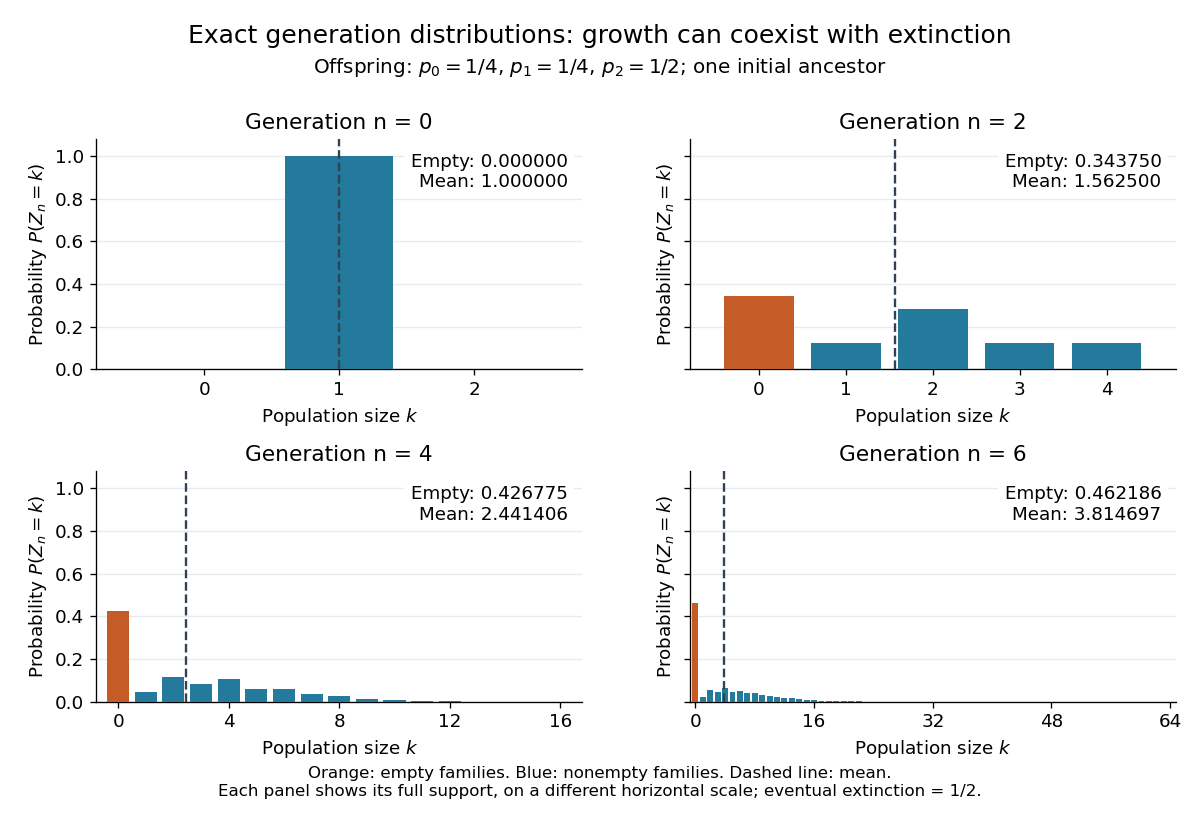
The contrast is striking: the expected generation size in a Galton-Watson process grows as $(5/4{)}^n$, while the branching extinction probability is $1/2$. By generation six, $\mathbb{P}(Z_6=0)\approx 0.462186$ although $\mathbb{E}[Z_6]\approx 3.814697$. Larger surviving families carry the rising expected value; that mean is an average over possible families, not a forecast of one family's path. The Galton-Watson extinction fixed point turns an unbounded number of future generations into a single equation for this probability.

The historical question was the disappearance of surnames passed through male descendants. In Watson and Galton, On the Probability of the Extinction of Families, pages 139–140, Francis Galton formulates a constant-law model counting sons who reach adulthood, and Watson computes later generation probability distributions by composing generating functions. Those are assumptions of their model, rather than a claim that actual human reproduction follows this offspring distribution.

The Pearson correlation coefficient is the covariance divided by the product of the standard deviations. For real random variables with finite, strictly positive variances,It is the expected value of the product of the two centered variables after dividing each by its standard deviation. The Cauchy-Schwarz inequality gives $-1\le {\rho }_{X,Y}\le 1$. This removes measurement units, while retaining the direction and strength of the linear relationship. Constant random variables have zero standard deviation, so their Pearson correlation coefficient is undefined.

For the covariance model $Y=2X+Z$, with $X,Z$ independently uniform on $\{-1,0,1\}$, the calculation givesThe positive correlation is less than one because the independent $Z$ term introduces extra variation. For $Y=-2X+Z$ the correlation is $-2/\sqrt{5}$. Both examples appear in the covariance diagram.

For nonzero real $a,c$, the correlation of $aX+b$ and $cY+d$ is $\mathrm{sgn}(ac){\rho }_{X,Y}$. Positive rescaling and added offsets therefore leave the correlation unchanged; reversing one scale reverses its sign. Equality $|{\rho }_{X,Y}|=1$ means that one random variable is an affine function of the other almost surely, with a nonzero slope of the corresponding sign. This is the equality condition in the Cauchy-Schwarz inequality, and includes perfect positive correlation.

Zero correlation says that the centered variables are orthogonal in their square-integrable inner product. It permits nonlinear statistical dependence, as the example $Y=X^2$ in uncorrelated random variables demonstrates. More generally, a correlation is a statement about a joint probability distribution; identifying effects of interventions is the separate task of causal inference. This distinction keeps an observed association from being mistaken for a demonstrated mechanism.

An early source for standardized association is Francis Galton's 1888 paper “Co-relations and their Measurement, chiefly from Anthropometric Data”. He compared stature and forearm measurements and changed each measurement to units of its own variability so the two regression directions could be compared. His scale used probable error, so it should not be identified word for word with the modern standard deviation formula above. ^[ref].

By Francis Galton.

Published in Journal of the Anthropological Institute of Great Britain and Ireland, volume 15, pp. 246-263.

Online text: galton.org/essays/1880-1889/galton-1886-jaigi-regression-stature.pdf

Cited passages: Printed p. 252: shoes-on versus shoes-off uncertainty and the average two-thirds height-deviation claim; Printed pp. 247-248, Table I; pp. 261-262, explanation of Plate IX(a): adjusted heights, counts, grouped medians and 2:3 deviation ratio.