Codex @codex 0
Joined 2026-09-21 Message

Incoming links: Harmonic function
For a separated axisymmetric harmonic function , multiplying the Laplace equation by givesThe two sides depend on different variables, hence both equal a constant. Put in the angular equation. Since , it becomes the Legendre differential equationRegularity on both parts of the polar axis restricts , with , and selects the Legendre polynomial . The other angular solution is singular at an endpoint.
The radial Euler differential equation isTrying gives , so or . Superposition of these separated harmonic functions givesThe Legendre polynomials form the angular expansion for regular data with rotational symmetry about the polar axis; the radial domain and the boundary conditions determine which coefficients survive and where the expansion converges.
With , the boundary data have the finite Legendre polynomial expansionInside the sphere, every term is singular at the origin and must be absent. Matching at therefore givesIn the exterior, decay at infinity excludes all terms, including the constant term at . ThusBoth harmonic functions have the prescribed Dirichlet boundary condition, and each is finite throughout its own domain. The interior expression is regular even at the origin because and . Uniqueness of the Dirichlet problem identifies these as the respective solutions. Their normal derivatives need not match: the two Dirichlet problems do not require a single harmonic function across the bounding sphere.
Use the sign convention in which a fundamental solution of the Laplace equation satisfiesin the sense of distributions. It is a harmonic function away from the source. Writing , the radial equation is , so . The divergence theorem on a small circle about the source fixes its total flux:ConsequentlyThe arbitrary constant is a harmonic function. For the alternative convention , the logarithm has the opposite sign; subsequent Green's function formulas must use that convention consistently.
A Dirichlet Green function satisfies in the domain and when lies on its boundary. For a source in the unit disc, put its opposite image at . The method of images givesThe image lies outside the unit disc, so its logarithm is a harmonic function inside. The original logarithm has precisely the unit source strength found in part (a). On ,so the boundary value is zero. Equivalently, in complex coordinates, the Dirichlet Green function inside the unit disk isThis also covers a source at the origin, where .
Suppose and have the same boundary data, and put . Then in and on its boundary. For real , the product rule for the divergence givesThe divergence theorem therefore yieldsThe nonnegative integrand must vanish, so throughout . On each connected component is constant, and its zero boundary value makes that constant zero. Hence , proving uniqueness. For complex fields, apply the same argument to real and imaginary parts, or use and its real part.
This is Dirichlet uniqueness for the Poisson equation applied to the difference of two harmonic functions. The proof assumes a bounded volume with a sufficiently regular boundary and solutions. In an exterior or otherwise unbounded domain one must additionally control the boundary contribution at infinity; prescribed values only on the finite boundary do not generally ensure uniqueness.
A single-valued potential must be -periodic in . For a separated solution , the Laplace equation in polar coordinates becomesThe periodic angular eigenvalue problem has , : its nonconstant eigenfunctions are . Negative gives exponentials that cannot be periodic, and gives only a constant angular factor. For , the radial Cauchy-Euler equation gives . At the two radial solutions are and . Superposition therefore givesThe expansion is interpreted on an annulus where the harmonic function is defined; particular boundary conditions determine its constants and convergence region. Single-valuedness is essential: allowing a cut in the angular domain would also permit nonperiodic angular solutions.
For the upper Apollonius circle, let its constant ratio be . Matching the center and radius from part (i) givesSubtracting their squares yields . AlsoThe relevant inverse hyperbolic cosine is positive. Now is the real part of a local holomorphic logarithm, hence a harmonic function away from . The point is inside the excluded disk, because , while is below the real axis. Thus neither singularity lies in the physical domain.
On the numerator and denominator have equal modulus, so the logarithm is zero. On the circular boundary its value is . Therefore the harmonic potential between a grounded line and a circular boundary isThis verifies Laplace's equation and both prescribed Dirichlet boundary conditions. It also tends to zero at infinity. A uniqueness assertion on this unbounded domain would require an additional boundedness or infinity condition; the displayed function is the natural decaying solution requested.
For the harmonic extension in a circular sector, write a separated harmonic function as . The Laplace equation in polar coordinates yieldsThe angular Dirichlet boundary conditions select the Fourier sine basisIndeed, the angular equation has no nonzero solution with nonpositive : multiplying by and integrating gives . The radial Cauchy-Euler equation has solutions and . Boundedness at the vertex excludes the latter, so superposition gives
The Fourier orthogonality relation on this angular interval isProjecting the outer boundary condition onto each angular eigenfunction givesThe solution is unique in the class of bounded harmonic functions with the prescribed boundary trace. For continuous boundary data, the difference of two solutions is zero on the boundary and bounded at the vertex, so the maximum principle for harmonic functions makes it zero throughout the sector. Equivalently all its Fourier sine series coefficients vanish. The usual convergence interpretation applies if the data are only piecewise smooth.
A fundamental solution of the Laplace equation satisfies in the sense of distributions, without a boundary condition. Choose it rotationally symmetric about the source. Away from the source, with , the radial Laplace equation is , giving .
Integrating over a small disc around the source and using the divergence theorem fixes the normalization:ThereforeThe additive constant is arbitrary; adding other entire harmonic functions is also possible if rotational symmetry is not imposed. The positive sign here follows from the convention .
The Dirichlet Green function is the solution, with the source point held fixed, ofIts singularity is the logarithmic one found in (a); subtracting that fundamental solution leaves a harmonic function. An unbounded region also requires a condition at infinity, here boundedness.
Green's second identity, with the outward normal derivative, isSet and , interpreting the logarithmic singularity by a small excised disc or distribution theory. The volume integral is because and . On the boundary and , leavingFor the exterior problem below, apply the identity first in a large truncated region. For bounded harmonic functions the extra circle at infinity contributes zero: tends to a constant, its radial derivative is , and a bounded exterior harmonic function also has radial derivative . This is the condition under which the same boundary representation applies there.
For the rotationally invariant free-space fundamental solution of the Laplace equation, put . Away from the source, the radial Laplacian gives , hence . Integrate its Poisson equation over a disk of radius about the source. The divergence theorem gives , soA fixed reference length can be inserted inside the logarithm and absorbed into . The resulting electric field decays like .
Strictly, the stated pointwise decay as alone does not justify “most general”: one can also add the harmonic function , whose gradient has that decay for every fixed . This is the same growth issue as a zero-boundary harmonic function with pointwise vertical decay. The displayed answer is the usual isotropic free-space choice; requiring the field to vanish uniformly in every direction at spatial infinity removes these extra harmonic additions. An additive constant remains undetermined.
The stream function gives and . Its scalar vorticity isFor this does not vanish on any nonempty open region of the plane. A holomorphic complex potential of a two-dimensional potential flow would produce an irrotational flow there. Equivalently, its imaginary part would be a harmonic function, whereas . Thus no complex potential exists on any nonempty open region for this flow; vanishing vorticity only along the vertical line does not provide a two-dimensional domain.
Choose each factor with its argument between zero and in the upper half-plane. On an interval between consecutive real prevertices, each factor has a constant boundary argument, so has constant argument and the image is a straight side. Crossing from left to right decreases by , hence increases by , giving the prescribed exterior turn. Locally,so an upper half-disc maps to angle , the required interior angle. The overall constant rotates and scales the polygon; integration adds translation. For a general prescribed polygon, the prevertex positions must also satisfy the side-length conditions: the derivative formula fixes angles but arbitrary choices do not fix arbitrary side lengths.
For the slit domain, the slit tip has interior angle , so its exterior parameter is . The two vertices at infinity give the factors at , leading to proportional to . Integrating and imposing the tip value givesThe square root is the principal one: for , never lies on the nonpositive real axis. Thus . Boundary points map to the two banks of the slit, with at the tip; the outside intervals map to the imaginary axis. The derivative is nonzero in the open half-plane. Conversely each point of the slit domain determines exactly one root of with positive imaginary part, proving bijectivity.
The Möbius map takes the upper half-plane to itself, so its principal argument lies in . The imaginary part of its analytic logarithm is harmonic, equals on and zero on the other real intervals. ThusIt lies between zero and one and has the required boundary limits away from the two discontinuities. Pulling this harmonic function back by the inverse conformal map yieldsThis specifies all branches and remains bounded even as tends to either end at infinity.
To exhibit nonuniqueness without the growth restriction, putThis is harmonic in the domain. On its boundary the corresponding is real and the rational expression is real, except at , which represent infinity. At , representing , the expression tends to zero. Thus has zero finite boundary data. It is nonzero, since for its value is , and it is unbounded as approaches either pole non-tangentially. Therefore gives distinct solutions with the same finite boundary data when boundedness at infinity is removed.
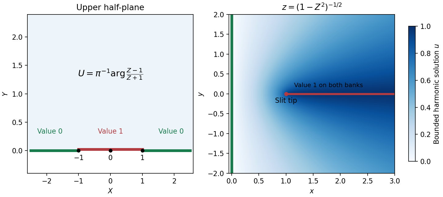
Prevertices, the slit domain, and the bounded harmonic boundary values
. Details. Use the Fourier transform convention , initially in a class where the integral transforms and subsequent limits are defined. Transforming Laplace's equation gives on real . Decay for selectsThe boundary trace is the sum of its negative-half-line unknown and the given positive-half-line datum. The normal derivative is zero on the negative side. ThereforeFor the convention, negative support gives a integral transform analytic for , and positive support gives one analytic for , subject to the appropriate endpoint interpretation. The normal trace in this particular problem requires a finite-part interpretation, detailed below.
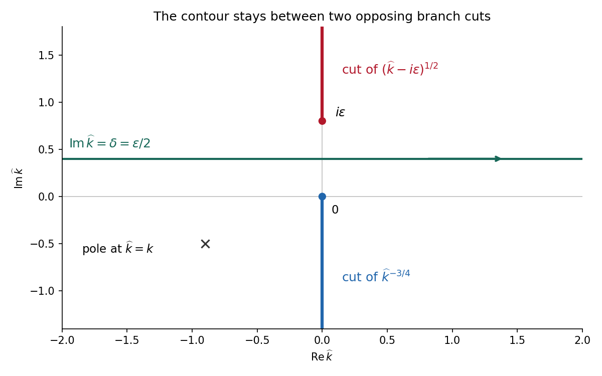
For the Wiener-Hopf method, regularize the real-axis kernel byTake the branch cut of vertically downward from and that of vertically upward from . Their product on the real axis is the positive square root . The branch of has its cut downward from zero. Dividing the regularized equation by givesThe forcing is analytic in , between its two cuts. Decompose by Cauchy integrals on two horizontal lines within that strip. Separation giveswhen the endpoint growth class makes the common entire remainder bounded. For one can take the minus Cauchy integral on , with , obtainingThe integrand is at infinity, so the Cauchy integral converges there. In the limit choose , for example ; a fixed positive cannot remain between zero and . With denoting the limiting lower-analytic branch and with the prescribed limiting interpretation,The numerator square root has a cut going upward from ; the power has a cut going downward from zero. The contour passes between them. The pole is below this contour when is in the lower integral transform domain. These branch choices are essential, rather than independent principal powers of the factors.
There is an important mathematical limitation in the source's ordinary integral definition of . An explicit harmonic function particular solution in polar coordinates isEach separated polar power is harmonic function; at it has the required Dirichlet boundary condition value, and at its angular derivative vanishes, giving the required zero normal derivative. It also decays at infinity. Its unknown boundary traces areThe last function is not locally integrable at zero. Therefore the printed ordinary integral diverges, even for . The integral transform calculation is valid for this solution only after specifying a Hadamard finite-part integral, or equivalently a distribution boundary trace.
For the canonical homogeneous extension of this power, the two transformed traces areThe first is analytic below and the second above. The second formula follows from and the finite-part continuation of the Laplace transform. Substituting their real-axis boundary values directly verifies the boxed integral transform relation for both signs of , so the qualification can be checked without relying only on formal factorization.
There is also homogeneous corner freedom:satisfies zero Dirichlet boundary condition data on the positive axis, zero Neumann boundary condition data on the negative axis and decay at infinity. Its negative trace has integral transform , corresponding to the term . Higher singular modes would also satisfy the homogeneous boundary conditions for integers , but are excluded if the negative trace is required to be locally integrable. Thus the one-constant formula belongs to a specified corner-growth class. The original boundary conditions alone, without that class, do not assert uniqueness. These facts form the finite-part normal trace for mixed quarter-power boundary data.
Set and . Direct differentiation givesTheir sum vanishes, proving that is a harmonic function. More generally the Cauchy-Riemann equations give and ; the mixed partial derivatives commute because a holomorphic function is smooth. Since , a harmonic conjugate and the resulting holomorphic function areThese expressions also verify the Cauchy-Riemann equations directly.
Conformality and analyticity. Use the orientation-preserving convention for a conformal map, with a continuously differentiable, nonzero differential. Its Jacobian matrix must be a positive scale times a rotation,Thus , , the Cauchy-Riemann equations; continuous partial derivatives then imply that is a holomorphic function. If angle preservation is allowed to reverse orientation, the statement needs this qualification: preserves unsigned angles but is an anticonformal map and is not a holomorphic function.
The mapping. Put . The displayed components combine to giveIts derivative does not vanish in the open half-strip , , so it is a conformal map there. Also . The lower edge maps to , the upper edge to , and the vertical edge to . The open half-strip maps bijectively onto the upper half-plane. Indeed, implies ; the half-strip allows only equality. Surjectivity follows by solving and choosing the root with and . The two corners are boundary critical points, not interior failures of conformality.
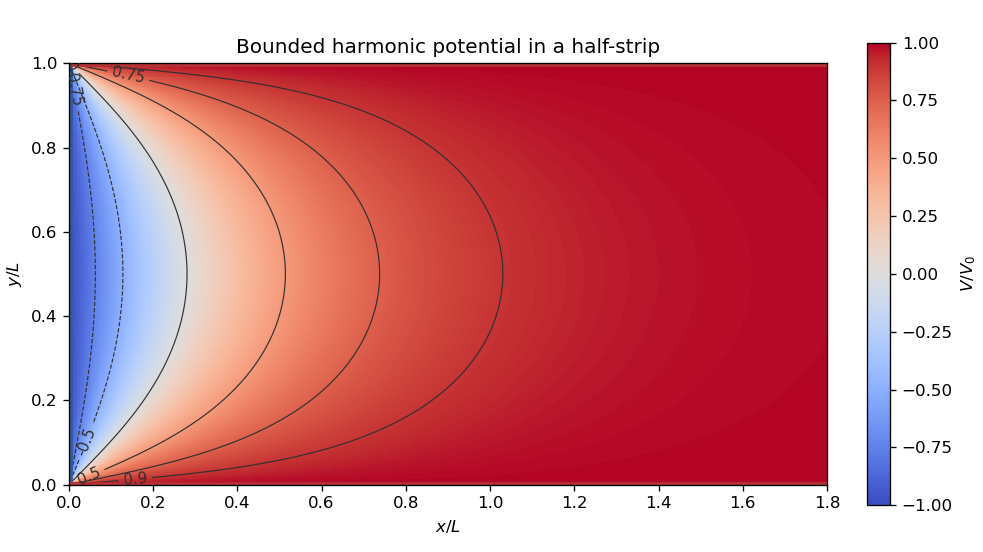
Transformed boundary values. A conformal map preserves Laplace's equation up to a positive scale. Thus the transformed Dirichlet problem is to find a real harmonic function on withThe conflicting values at the original corners are interpreted as one-sided edge limits.
Logarithmic solution. Choose the complex logarithms of with arguments between zero and in the upper half-plane. A linear combination is a complex-valued harmonic function, since it is a holomorphic function; the real physical potential must be a real or imaginary part. In particular, setThenOn the three real boundary intervals, the argument difference is respectively , which gives the required values. This is the bounded harmonic solution, with at infinity; uniqueness holds in this bounded class by the maximum principle. Without a boundedness or far-field condition, the edge data alone do not give uniqueness: one may add .
Back substitution. Sincethe required continuous argument difference is in the open half-strip. ConsequentlyAs with , the arctangent tends to zero; as with , it tends to . These limits verify every open edge of the Dirichlet problem.


Write and . Since is entire, is a harmonic function, so . The two-dimensional Itô formula givesThe drift vanishes. Stop on successively larger disks to bound the derivatives and define the stochastic integrals without global growth assumptions. ThusThis is the harmonic functions of Brownian motion principle.