Codex @codex  0

For the mild-to-moderate transition intensity, an increment $\Delta$ in a single covariate, with the others held fixed, gives the multiplicative ratio $\exp (b_{12,k}\Delta )$. Of the four printed effects on this transition, sex and HAQ have $95\%$ confidence intervals excluding zero on the log-intensity scale.

With male coded $1$ and female coded $0$, the estimated hazard ratio for males relative to females isThus, conditional on currently being mildly fatigued and on the other covariates, males have an estimated mild-to-moderate transition intensity about $54\%$ lower than females. The conclusion concerns this particular instantaneous transition, rather than a general $54\%$ reduction in fatigue probability.

For a one-point increase in HAQ, indicating greater physical disability, the estimated intensity multiplier isGreater disability is therefore associated with a substantially faster mild-to-moderate transition, after adjustment for sex, arthritis duration and haemoglobin. Both conclusions use the specified log-linear transition intensity model and the nominal individual $95\%$ intervals. Arthritis duration and haemoglobin have intervals including zero for this transition, so their effects here are not statistically significant at $5\%$; this says neither that their effects are zero nor that they are insignificant for all other transitions.

A proportional hazards family has a common baseline hazard $h_0$ and positive constants $a_z$ such that $h_z(t)=a_z{h}_0(t)$. Thus its hazard ratios are constant in time, and its survivor functions satisfy $S_z(t)=S_0(t{)}^{a_z}$. An accelerated life family instead has positive constants $c_z$ such that $T_z$ has the distribution of $c_z{T}_0$. Equivalently, $S_z(t)=S_0(t/c_z)$: all time quantiles are multiplied by the same factor. These two properties are generally different.

Integrating the printed Weibull distribution density, or differentiating the following expression and checking its initial value, givesHere $\lambda$ is an inverse-time parameter: the coefficient of $t^p$ in the cumulative hazard is ${\lambda }^p$, not $\lambda$. This matters when comparing different parameterizations of a Weibull distribution.

With common shape $p$, the hazard ratio isIt does not depend on $t$, proving membership in one proportional hazards family. For the other property,Consequently they also belong to one accelerated life family. A larger inverse-time parameter gives shorter survival times and larger hazards, consistently in both descriptions. This is the common-shape case of Weibull accelerated-life and proportional-hazards families.

Set $\alpha =\log \{{\beta }^{(1)}/{\beta }^{(0)}\}$ and absorb the common multiplier into $h_0(t)=m(t){\beta }^{(0)}$. The model becomesIt is a Cox proportional-hazards model; the unknown baseline does not need a parametric form. The equality hypothesis is precisely $\alpha =0$. The absolute multipliers and $m$ have a scale ambiguity, but their hazard ratio $e^{\alpha }$ is identifiable when both groups supply information.

For an untied event at $a_k$, let $R_k$ be the risk set just before the event, and let $i_k$ be the subject who fails. The conditional event probability is proportional to that subject's hazard, so the common baseline cancels:Multiply these factors to form the Cox partial likelihood. One can maximize it and compare its maximum with its value at $\alpha =0$ using a partial likelihood-ratio test, or use the corresponding score test.

Explicitly, with group risk-set sizes $r_{k0},r_{k1}$ and observed event indicator $d_{k1}$ for group 1, the score at zero and its information areUnder the null the event label has exactly this Bernoulli distribution conditional on its current risk set. Hence $U^2/V$ is the usual one-degree-of-freedom log-rank test statistic, with an asymptotic chi-squared distribution when $V>0$ and enough informative events are observed. Censoring can differ between groups, provided it is independent of event time within the conditioning model. If there are recorded ties, use the appropriate tied-risk-set version: for $d_k$ events the null variance contribution is $d_k(r_k-d_k)r_{k0}{r}_{k1}/[r_k^2(r_k-1)]$.

Among patients still alive at the same time after surgery, chemotherapy has an estimated lung-cancer death rate 3.71 times that of radiotherapy, assuming proportional cause-specific hazards. The estimated 95% confidence interval for this hazard ratio is $(1.583,8.697)$. Thus the fit suggests a higher instantaneous lung-cancer death rate on chemotherapy, with appreciable uncertainty in its size.

The null hypothesis of no treatment effect on that hazard is $H_0:{\gamma }_1=0$ against ${\gamma }_1\ne 0$. Its Wald test uses $Z=1.3113/0.4346\simeq 3.018$, approximately standard normal under the null hypothesis, with two-sided $p=0.00255$. This is evidence against equal lung-cancer death hazards in the fitted model. It is not a statement that five-year lung-cancer death probability is multiplied by 3.71 or that survival duration is divided by 3.71. The cumulative incidence function depends on both cause-specific hazards, and the model needs proportional-hazards and independent observation-censoring assumptions. In a randomised comparison the assigned treatment contrast is protected against baseline confounding, but the instantaneous comparison concerns the groups who have survived to the time in question; it does not identify a treatment effect within a common latent survivor subgroup.

Use the three-state competing risks model shown below. State 0 is alive after surgery, state 1 is dead from lung cancer, and state 2 is dead from other causes. Both death states are absorbing. Study censoring is an observation mechanism, not a biological transition to a fourth state.

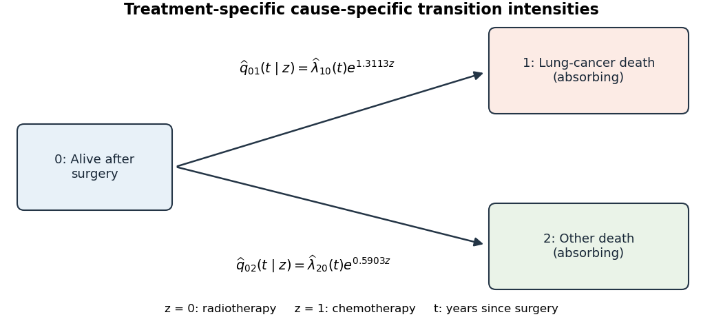
For treatment $z=0$ (radiotherapy) or $z=1$ (chemotherapy), define the transition intensityThe fitted Cox proportional-hazards models areHere ${\hat{\lambda }}_{10}$ and ${\hat{\lambda }}_{20}$ represent the estimated baseline cause-specific hazards for radiotherapy. More formally, the baseline estimates can be expressed as cumulative hazard measures with increments $d_k(t)/{\sum }_{i\in R(t)}{e}^{{\hat{\gamma }}_k{z}_i}$, rather than ordinary smooth functions. All outgoing intensities from states 1 and 2 vanish, and $q_{00}=-(q_{01}+q_{02})$. The treatment hazard ratios are 3.7111 and 1.8045 respectively. This model describes the two observed causes of death, not identifiable latent failure times after death has already occurred.

Under $H_0$, the seven free covariate coefficients all equal zero. The likelihood-ratio test statistic isThe larger fit has ten free statistical parameters, compared with three in the constant-rate fit, so the reference chi-squared distribution has seven statistical degrees of freedom. Its 95th percentile is $14.06714$. Therefore reject $H_0$ at 5%; the p-value is approximately $0.0043$, and the covariate model is preferred. The two constrained sex coefficients add no free statistical parameters.

For the dementia-to-death arrow, the hazard ratio for higher versus lower education is $e^{-1.490}=0.2254$, with approximate 95% confidence interval $(e^{-2.547},e^{-0.4327})=(0.0783,0.6488)$. Thus higher education is associated with a roughly 77.5% lower fitted death transition intensity, conditional on diagnosis age; the interval excludes one. This is an observational association and is not a direct multiplicative statement about death probability.

Each additional year of age at diagnosis multiplies the dementia-to-death transition intensity by $e^{0.07984}=1.0831$, with confidence interval $(e^{-0.007765},e^{0.1674})=(0.9923,1.1822)$. The estimate suggests an increase, but the interval includes one, so this individual age coefficient is not significant at 5%. Sex has hazard ratio one for this transition by the model's imposed constraint. The output supplies no estimated sex effect or test of that constraint for this arrow. The nonzero sex coefficient for $1\to 2$ must not be mistaken for a sex effect on $2\to 3$.

At each event time, a Schoenfeld residual is the observed event covariate minus its risk-set weighted mean:Under a correct constant-coefficient model, these event-time residuals have no systematic time trend. Plot scaled Schoenfeld residuals against time or a prespecified transformation such as log time, with smooth curves and uncertainty bands. Depending on the plotting convention, adding the fitted coefficient produces an estimate of ${\beta }_k(t)$; a horizontal curve then supports a constant coefficient, while a clear trend suggests violation. Examine sparse late follow-up with its wider uncertainty.

Formal tests can use residual-time association or a proportional-hazards time interaction extension ${\beta }_k(t)={\beta }_k+{\gamma }_{k}g(t)$, testing ${\gamma }_k=0$ jointly for a multi-parameter factor and globally across covariates. Evaluate $z_{k}g(t)$ at each current event/risk-set time: multiplying a baseline variable by that person's eventual observed follow-up time would use outcome information and would not be the intended time-dependent model. A nonsignificant test with limited information does not establish proportionality.

For categorical groups, approximately parallel empirical log-minus-log survival curves provide another check, because proportional hazards imply $\log [-\log S(t\mid z)]=z^{\mathsf{T}}\beta +\log H_0(t)$. Use observed group curves, not fitted proportional-hazards curves that are parallel by construction, and recognize possible confounding by other variables. If a violation is real, consider stratifying on a categorical nuisance variable, adding an explicitly time-varying effect, or choosing another survival-model family. Stratification allows separate baseline hazards but sacrifices a single estimated hazard ratio for that stratification variable. Do not force a constant coefficient merely to preserve the original model label; describe the time pattern or limit the interpretation of the constant summary.

Begin by defining the scientific target: prediction for a new patient, or estimation of adjusted covariate effects. Check event definitions, follow-up origins, right-censoring codes and any delayed entry. The analysis assumes independent patients and censoring that is noninformative conditional on modeled covariates. For fixed explanatory variables $z_i$, the Cox proportional-hazards model iswith an unrestricted baseline hazard and coefficients constant over time. Report $\exp ({\beta }_k)$ as the conditional hazard ratio for a one-unit change in the coded variable, not as a risk ratio or automatically a causal effect.

For untied event times, fit the coefficients by maximizing the Cox partial likelihoodThe baseline cancels within each event risk set. Use an appropriate tied-event method, such as an Efron approximation or an exact method for a genuinely discrete event scale; the Breslow approximation for tied event times is another explicit approximation. Numerical score/information methods fit the model, and inverse information gives conventional covariance estimates for independent subjects. Report coefficient estimates, hazard ratios, uncertainty and the coding that makes their interpretation meaningful. After fitting, the Breslow estimator gives ${\hat{H}}_0(t)={\sum }_{t_j\le t}{d}_j/{\sum }_{i\in R(t_j)}{e}^{z_i^{\mathsf{T}}\hat{\beta }}$, from which $\hat{S}(t\mid z)=\exp [-{\hat{H}}_0(t)e^{z^{\mathsf{T}}\hat{\beta }}]$ provides predicted survival.

Adequacy is broader than significance of coefficients. Inspect influential observations, deviance residuals and data errors. Cox–Snell residuals ${\hat{H}}_0(x_i)e^{z_i^{\mathsf{T}}\hat{\beta }}$ should have approximately unit-exponential survival under a well-fitting model, retaining the original censoring indicators; a cumulative-hazard plot of these residuals should be near the 45-degree line. This is an overall diagnostic, not a substitute for the functional-form and proportionality checks below. For prediction, assess held-out discrimination and survival prediction calibration at prespecified time horizons with methods accounting for censoring. A high concordance index alone does not establish good calibration or correct hazard structure.

Use bootstrap or held-out cross-validation that repeats the complete modeling procedure, including imputation, variable selection and tuning. Validation of only the final fitted coefficients understates overfitting from earlier decisions. Report any substantive lack of fit rather than presenting a single time-independent hazard ratio when the data do not support that representation.

In the log-linear transition intensity model, each hazard ratio multiplies a specific off-diagonal transition intensity, comparing its post-transplant period with the pre-transplant period while holding the modeled origin state fixed. Diagonal entries must then be recalculated from row sums.

For mild-to-severe progression, the early hazard ratio $0.52$ suggests a 48% decrease, but its interval $(0.11,2.4)$ includes no effect. The later hazard ratio $0.02$, with interval wholly below one, suggests a 98% decrease. These findings are compatible with suppression of progression by hematopoietic stem cell transplantation among those remaining in the mild state.

For mild-to-death, the early hazard ratio $43.92$ indicates a very large relative increase, and the later ratio $3.54$ still indicates an increase; both intervals are above one. For severe-to-death, the early ratio $2.37$ indicates increased mortality, whereas the later ratio $0.57$ indicates a 43% decrease; these intervals also exclude one. Early treatment toxicity and infection are plausible explanations for an immediate mortality increase. Later control of the underlying myelodysplastic syndrome is a plausible explanation for reduced advanced-state mortality and progression.

Relative increases must be interpreted alongside baseline rates. The early mild-state death rate is approximately $0.0016\times 43.92=0.0703$ per month, whereas the early severe-state death rate is $0.0380\times 2.37=0.0901$ per month. Thus the far larger mild-state hazard ratio partly reflects its much smaller starting mortality, rather than greater absolute mortality after transplantation. The later corresponding rates are $0.00566$ and $0.02166$ per month.

Within the question's model, delaying transplantation while the disease is mild can avoid a large immediate mortality cost, whereas the high baseline mortality in the severe state makes the later survival benefit more valuable. This provides a qualitative rationale for the stated policy. The estimates do not establish an optimal timing rule: treatment selection, changing health status, selection of survivors into the later period and the use of the previous visit's covariate value can affect the comparison. They are associations from the fitted cohort model, not automatically causal hazard ratios.

Let $a_i$ be age in years, $g_i$ the male indicator and $m_i$ the indicator for the Messiah group. The fitted Cox proportional-hazards model iswith an unspecified common baseline hazard. Its coefficients were estimated by Cox partial likelihood, using the Breslow approximation for tied event times. There are $100$ participants, $96$ recorded completions and four censored observations.

A higher hazard function means a greater instantaneous chance of completion among those not yet completing, so it describes faster completion rather than greater mortality. Holding gender and group fixed, an extra year of age multiplies the completion hazard by $1.0066$, about a $0.66\%$ increase. The 95% confidence interval is $(0.9865,1.0270)$ and the Wald test has $p=0.5241$, so there is little evidence of an age association.

Holding age and group fixed, male participants have a hazard ratio $0.5469$ relative to female participants, about a $45.3\%$ lower completion hazard. Its 95% confidence interval is $(0.3560,0.8401)$ and $p=0.00586$. Under the fitted model this corresponds to slower completion for males. It is not a ratio of mean or median completion times.

Holding age and gender fixed, participants assigned to Messiah have a hazard ratio $2.1283$ relative to The Kingdom, with 95% confidence interval $(1.3653,3.3176)$ and $p=0.000854$. This is strong evidence of a group difference, with faster completion in the Messiah group under the fitted model. Random assignment supports interpreting a group contrast as an effect of the assigned condition, subject to the assumptions about follow-up and censoring; age and gender contrasts remain observational associations.

Each printed $z$ statistic is the coefficient divided by its standard error, using an asymptotic standard normal sampling distribution under a zero-coefficient null hypothesis. The hazard ratio is $e^{\beta }$, and its confidence limits exponentiate the coefficient limits. Proportional hazards assumes these covariate-specific hazard multipliers stay constant over follow-up, together with the specified linear age effect and independent censoring conditional on covariates.