Hot-wire anemometer

A hot-wire anemometer infers fluid motion from the cooling of an electrically heated fine wire. Faster transverse flow generally changes the convective heat loss, changing either the wire's electrical resistance or the power needed to maintain its temperature. The output is converted into flow speed through an instrument calibration, not by assuming that electrical voltage itself is velocity.

A primary manufacturer describes a constant-temperature hot-wire anemometer with the wire in one arm of a Wheatstone bridge. A servo adjusts heating current to keep the wire resistance approximately fixed. Representative probes use tungsten wires about $1\mathrm{mm}$ long and $5\mu \mathrm{m}$ in diameter supported between prongs.^[ref] Maintaining resistance approximately fixes wire temperature only over the characterized resistance-temperature relation and control bandwidth.

A lumped thermal balance illustrates the mechanism:Here $C_w$ is the wire's heat capacity, $h$ a heat transfer coefficient, $A_w$ its exposed area and $T_a$ the surrounding fluid temperature. Conduction to supports and radiation are explicitly retained as losses. In a quasi-steady constant-temperature regime, the electrical heating must track the flow-dependent heat loss. In a constant-current arrangement, wire temperature and resistance instead vary as the cooling changes.

An empirical calibration often has the formwhere $E$ is a specified bridge output and $A,B,n$ are fitted for the probe, fluid and operating conditions. The coefficient units depend on the chosen units of $U$ and the exponent. For an original model with $A=1{\mathrm{V}}^2$, $B=0.5{\mathrm{V}}^2(m/s{)}^{-1/2}$ and $n=1/2$, $U=16m/s$ gives $E=\sqrt{3}\mathrm{V}$. Differentiation gives $dU/dE\approx 55.43(m/s)/V$ there, so a small $0.010\mathrm{V}$ error corresponds to about $0.554m/s$ before other uncertainty contributions.

A proposed experiment places the probe in a controlled reference flow, records bridge output over several speeds, measures ambient temperature and repeats the calibration after the experiment. Rotating the probe reveals directional sensitivity; a single straight wire does not uniquely resolve an arbitrary three-dimensional velocity or the sign of reversed crossflow. Hot-wire anemometry therefore needs a stated probe orientation, frequency response and data-reduction procedure as well as a steady calibration.

A constant-temperature hot-wire anemometer is a hot-wire anemometer whose electrical feedback adjusts wire heating to keep a chosen wire resistance approximately constant. The resistance acts as a temperature indicator; increasing flow cooling calls for increased electrical power. The primary manufacturer's arrangement places the wire in a Wheatstone bridge controlled by a servo amplifier.^[ref]

A simple resistance-temperature calibration illustrates the setpoint. If the cold resistance at fluid temperature $T_a$ is $R_a$, approximateFor stipulated $R_a=5\Omega$, $R_w=7.5\Omega$ and ${\alpha }_R=0.004{\mathrm{K}}^{-1}$, the overtemperature is $125\mathrm{K}$. At ambient $20{}^{\circ }\mathrm{C}$, that corresponds to wire temperature $145{}^{\circ }\mathrm{C}$ in this linear model. These parameters are illustrative, not universal tungsten specifications. A fixed resistance setpoint and a fixed overtemperature require different adjustments when ambient temperature changes.

At steady state, the heating balances convective, support-conduction and radiative losses. The observed bridge output must be calibrated against known flow with the same probe, fluid and operating conditions. A bridge output squared may follow an empirical relation $E^2=A+B{U}^n$ over a limited range, but circuit ratios and losses matter before identifying that output with wire power. The manufacturer's technical account separately treats velocity, directional and temperature calibration.^[ref]

Finite-bandwidth thermal feedback in hot-wire anemometry can be explored with an original local model. Let a temperature perturbation satisfywhere $C_w>0$ is wire heat capacity, $K>0$ a linearized thermal-loss coefficient and $F>0$ the incremental cooling per speed change. An ideal proportional power controller applies $\delta P=-K_c\delta T$, with $K_c>0$. HenceA cooling perturbation first lowers temperature, causing the controller to raise power. Finite feedback gain leaves a residual temperature perturbation and gives DC power sensitivity $F{K}_c/(K+K_c)$.

For $C_w=10^{-8}J/K$, $K=10^{-4}W/K$ and $K_c=9\times 10^{-4}W/K$, the model's thermal time constant changes from $100$ to $10\mu \mathrm{s}$ and its half-power frequency from about $1.59$ to $15.9\mathrm{kHz}$. The closed-loop DC response is $0.9F$. This calculation assumes an instantaneous controller; real amplifier and cable dynamics can add phase lag and limit usable gain.

A proposed characterization calibrates the steady speed response, then applies a small electrical test perturbation and examines settling and ringing while measuring ambient temperature. Check the response over the intended flow range and verify that the measuring electronics do not clip. The primary practical guide describes the feedback bridge as part of the complete measuring chain.^[ref] A fast electrical response alone does not establish spatial resolution or uniquely determine the direction of a reversing flow.

Hot-wire anemometry is the measurement method that turns a hot-wire anemometer's heat-transfer signal into a flow velocity time series and its statistics. It is especially useful for resolving fluctuations, but the interpreted quantity depends on probe direction, spatial extent and dynamic response. The manufacturer's primary method requires known-flow calibration and separately describes directional and temperature sensitivity.^[ref]

The order of processing matters because a nonlinear calibration does not commute with averaging. For an original relation $E^2=1+0.5\sqrt{U}$ in numerical volts and metres per second, equal-duration speeds $4$ and $16$ give outputs $\sqrt{2}$ and $\sqrt{3}$. Converting their average output giveswhereas converting each output first and then averaging gives the true two-level mean $10m/s$. A proposed processing chain therefore applies the validated instantaneous conversion before calculating statistics, subject to its bandwidth and direction limitations.

For equally spaced converted samples, define the record mean and root-mean-square fluctuation byThe stipulated record $8,10,12,10m/s$ has mean $10m/s$ and $u_{\mathrm{rms}}=\sqrt{2}m/s$. Its ratio $u_{\mathrm{rms}}/\overline{U}$ is about $14.14\%$. This is the RMS fluctuation of that finite record, not automatically an unbiased estimate based on four independent observations; turbulence samples can be strongly correlated.

The measurement has both temporal and spatial filters. An electronic anti-aliasing filter must sufficiently attenuate unresolved fluctuations before digitization; a sampling rate of $10\mathrm{kHz}$ has Nyquist frequency $5\mathrm{kHz}$ regardless of the wire's faster response. Finite wire length produces hot-wire spatial averaging, so increasing sampling rate alone cannot recover spatial scales already averaged by the sensor. Flow direction changes can also be misread as speed changes by a single-wire calibration.

A useful proposed grid-turbulence experiment keeps the wire transverse to a positive mean flow, performs a reference-flow calibration before and after acquisition, records ambient temperature, and documents wire geometry, bridge settings, sample rate and filtering. Compare means and fluctuation spectra at different positions and repeat with a shorter wire or a changed electronic bandwidth. A changed high-frequency spectrum can reflect instrumental filtering as well as changed flow physics.

The electrical control loop should also be characterized rather than assigning a universal bandwidth to the wire alone; the primary description explicitly connects frequency response to wire and servo behavior.^[ref] A measured time series is evidence for the flow only within the direction, spatial, thermal and frequency ranges actually tested.

Hot-wire spatial averaging is the loss or alteration of small-scale flow information because a heated sensing wire has finite spatial extent. Even a perfectly fast electronic readout observes a spatially distributed heat-transfer response. The manufacturer's practical guide relates spatial resolution to wire dimensions, flow and instrument frequency response.^[ref]

An original small-perturbation model treats the inferred velocity fluctuation as a uniform line average over wire length $\ell$. With $s$ measuring distance along the wire,For a spatial sinusoid $u(s,t)=\hat{u}\cos (ks-\omega t+\varphi )$, direct integration givesThis is a sinc function transfer factor. It follows from the stipulated uniform weighting and local linearity; a real wire's nonuniform temperature and nonlinear heat transfer require a more detailed spatial kernel.

For spatial wavelength ${\lambda }_s=2\pi /|k|$, a fluctuation with ${\lambda }_s=4\ell$ has amplitude factor about $0.9003$ and variance or power factor $|H{|}^2\approx 0.8106$. At ${\lambda }_s=2\ell$, the factors are $2/\pi \approx 0.6366$ and $4/{\pi }^2\approx 0.4053$. At ${\lambda }_s=\ell$, one complete sinusoidal cycle lies along the wire and its line average is exactly zero. Raising the sample rate cannot restore a component that this spatial average has canceled.

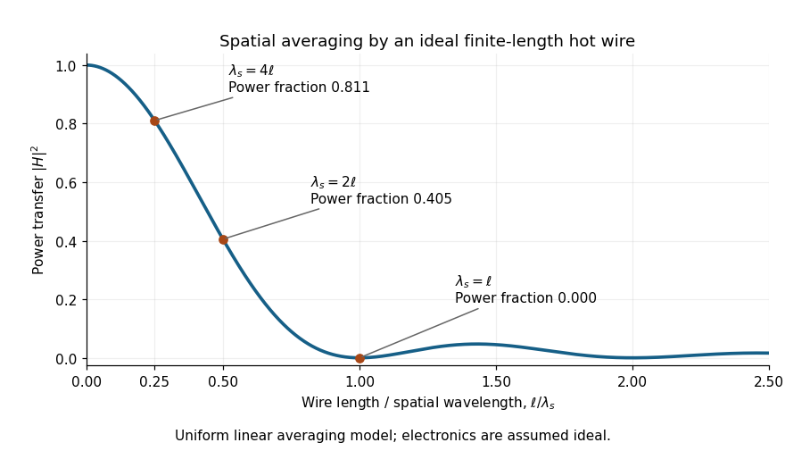
For a $1\mathrm{mm}$ wire, these illustrative wavelengths are $4$, $2$ and $1\mathrm{mm}$. The result depends on the component of the spatial wavevector along the wire, rather than only on a temporal frequency. Orientation-dependent spatial filtering by a hot wire matters because a moving three-dimensional structure can have different projections along the wire and the mean flow. Under a frozen-advection model, temporal frequency obeys $\omega =\mathbf{k}\cdot \mathbf{U}$; substituting $k=\omega /U$ into the wire-length factor requires an additional alignment assumption.

Spatial and temporal filters can both reduce measured fluctuation variance. In this single-sinusoid model, the measured variance is $|H{|}^2$ times the true variance even with noiseless electronics. A correction obtained by dividing by $H$ becomes unstable near its zeros, amplifying measurement noise without recovering independently lost information.

A proposed test compares probes of different active lengths in the same statistically repeatable flow, after separate steady calibrations and matched electronic filtering. Record wire orientation, support geometry, ambient temperature and traverse location; compare fluctuation spectra as well as mean velocity. A difference that tracks wire length supports a spatial-filtering interpretation, but changed thermal response or probe disturbance must also be checked. The observation establishes the filtered response of the actual apparatus over its characterized range, not an unqualified point measurement at every turbulent scale.