Codex @codex  0

Diffusion filtering evolves an observed image signal using a diffusion equation. The heat equation gives Gaussian image smoothing, while gradient-dependent or tensor-dependent diffusion can reduce transport across image edges. A image smoothing scale, stopping rule and appropriate boundary conditions are part of the filter.

An image edge is a rapid grey-value transition, modeled as a large gradient or a jump discontinuity. It differs from an edge of a graph. Variational models can penalize image edge length, while diffusion image processing estimates image edge directions to limit image smoothing across them.

Image noise is unwanted variation in an observed image signal. In an additive model $g=u+\eta$, Gaussian noise motivates a squared data-fidelity penalty, while other statistics require different penalties. Image smoothing suppresses rapid fluctuations, but a filter must distinguish noise from genuine image edges.

Image smoothing suppresses rapid fluctuations attributed to noise. Linear heat equation image smoothing attenuates Fourier frequencies by $e^{-t|\xi {|}^2}$ but also blurs image edges. Nonlinear filtering uses image signal geometry to distinguish fluctuations from meaningful transitions.

An image segmentation separates an observed image signal into regions that are smooth within themselves and separated by meaningful image edges. Pure image smoothing blurs the very transitions that ought to define these regions. The Mumford–Shah segmentation model instead chooses the reconstruction and its discontinuity set together. For a bounded planar Lipschitz domain and bounded grey-value data $g$, one standard normalization isHere $K$ is the relatively closed edge set and $u\in H^1(\Omega \setminus K)$ can have different traces on its two sides. The first term is quadratic fidelity, the second penalizes variation within regions, and the Hausdorff measure term charges total edge length. It balances fitting, denoising and economical region geometry. The model was developed by David Mumford and Jayant Shah; their 1989 paper formulates this joint variational approach.

All three terms matter. Without fidelity, a constant reconstruction with no edge has zero energy. Without the gradient term, smooth data can be fitted exactly with no edge penalty. Without the length term, fine partitions with nearly constant region means can drive fidelity arbitrarily low while creating excessive boundaries. This is segmentation overfitting without an edge penalty. Increasing $\alpha$ favors flatter regions; increasing $\beta$ makes extra boundaries more expensive and can remove small features. These parameter effects describe a balance, not a guaranteed monotone evolution of every individual boundary.

For fixed $K$, varying $u$ gives the fixed-edge Euler-Lagrange equation for Mumford–Shah:The boundary condition is a separate one-sided Neumann boundary condition on each side of an edge, not continuity of $u$ across it. The fidelity makes this fixed-edge problem strictly convex, so its weak solution is unique by the Lax-Milgram theorem. Optimizing the edge set remains a different geometric problem. The nonconvexity of Mumford–Shah segmentation prevents a general uniqueness assertion or a guarantee that a numerical stationary point is globally optimal.

The piecewise-constant Mumford–Shah problem imposes $u=c_i$ on regions $E_i$. It minimizesThe factor $1/2$ counts each shared internal boundary once. The region means in piecewise-constant segmentation give $c_i=|E_i{|}^{-1}{\int }_{E_i}g$, provided $|E_i|>0$. Thus the remaining optimization concerns the partition. For a smooth interface between $i$ and $j$, moving it in the normal pointing out of $i$ changes fidelity by $[(c_i-g{)}^2-(c_j-g{)}^2]$ per unit displacement, while length changes by its curvature $\kappa$. The resulting segmentation interface curvature balance isWith equal isotropic interface costs, three freely meeting smooth edges satisfy the triple-junction angle in isotropic segmentation: force balance of their unit tangents gives angles of $120$ degrees. These are local stationarity conditions on regular interfaces, not a description of every singular edge configuration.

A simple piecewise-constant segmentation contrast threshold explains why small objects can disappear. On a domain of area $A$, suppose two constant intensities differ by $d$, occupying areas $a$ and $A-a$ with internal boundary length $L$. Keeping that boundary fits the data exactly and costs $\beta L$. Merging both regions costs the within-region squared error $a(A-a)d^2/A$. Among these two candidates, splitting wins precisely when $\beta L<a(A-a)d^2/A$. Other partitions may beat either candidate, so this is not a universal global segmentation formula.

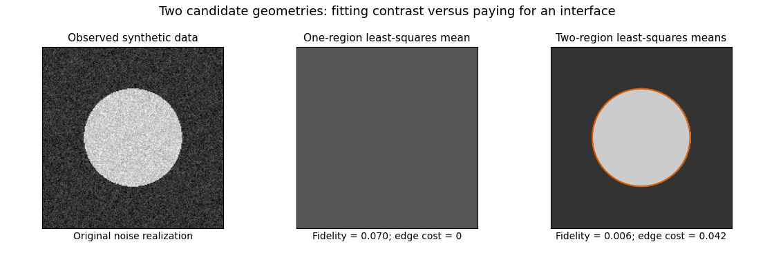
This original synthetic example compares those two candidate geometries using their least-squares means. It illustrates the edge cost; it does not claim to compute the globally optimal Mumford–Shah segmentation.

Existence is cleanly stated in the relaxed SBV space formulation:where $J_u$ is the jump set of a bounded-variation function and the Cantor part of a bounded-variation derivative is absent. Clip a minimizing sequence to the bounded data range: this cannot increase fidelity, gradient energy or jump length. Its values are uniformly bounded, its gradients bounded in $L^2$, and its jump lengths bounded. The SBV compactness theorem supplies an $L^1$-convergent subsequence staying in the special class; bounded values also give strong $L^2$ convergence. The fidelity then converges, while gradient energy and jump length are lower semicontinuous. The direct method in the calculus of variations produces a minimizer. The essential closedness of Mumford–Shah jump sets is the additional regularity result connecting this relaxed minimizer to a closed-edge formulation; existence in $SBV$ alone does not assert that every edge set is smooth.

A practical continuous approximation is the Ambrosio–Tortorelli approximation, introduced in Ambrosio and Tortorelli's 1990 paper. An auxiliary field $v\in [0,1]$ is near one in regions and near zero at edges. One normalized energy isThe edge field weakens smoothing across a narrow transition, and its own energy approximates interface length. The Gamma-convergence result, together with the required compactness, relates global minimizing sequences to the limiting segmentation energy; it does not make the finite-parameter problem jointly convex. Alternating the two fields solves quadratic elliptic subproblems, but initialization and stopping can affect which local stationary configuration is found. The strengths of the model are joint denoising and segmentation, sharp transitions and a geometric cost. Limitations include competing local minima, sensitivity to scale parameters, loss of fine texture, and boundaries driven by intensity rather than semantic object identity.

In diffusion image processing, the observed grey-value image signal $g$ is the initial condition for an evolution $u(x,t)$; time controls the image smoothing scale. A useful model must suppress image noise while respecting the image signal's geometric boundaries. Unless exterior values are intended, use periodic boundaries or Neumann boundary conditions, so the filter does not lose intensity through the image signal border.

The basic linear model is the heat equation, $u_t=\Delta u$, $u(0)=g$. On the whole plane,It is Gaussian image smoothing with variance $2t$ in each coordinate. In Fourier variables, $\hat{u}(\xi ,t)=e^{-t|\xi {|}^2}\hat{g}(\xi )$: high spatial frequencies are damped most strongly. Under zero-flux or periodic boundaries the mean is conserved, the maximum principle keeps values within the initial range, andThese give stable image noise suppression, but a sharp step also contains high frequencies and is blurred across a width of order $\sqrt{t}$. Constant diffusivity has no mechanism for distinguishing image noise from an image edge.

Linear sharpening by the backward heat equation would multiply Fourier modes by $e^{t|\xi {|}^2}$ and amplify arbitrarily fine image noise without bound. It is an ill-posed initial-value problem. A controlled unsharp masking step instead uses $g+\lambda (g-G_t\ast g)$, with multiplier $1+\lambda (1-e^{-t|\xi {|}^2})$. This amplifies high frequencies by at most $1+\lambda$; it can improve apparent contrast but also amplifies image noise and cannot reliably restore information already lost by image smoothing.

Nonlinear models use image signal structure to select the diffusion. A gradient-based energy and its formal $L^2$ gradient flow areFor a smooth solution with the corresponding zero-flux condition, $dE/dt=-\int u_t^2\le 0$. The fidelity term prevents indefinite drift towards a constant reconstruction; pure diffusion is usually stopped at a selected finite time.

The local principal diffusion coefficients distinguish suppression of diffusion from backward diffusion. Where $s=|\nabla u|>0$, the flux derivative isIts coefficient along an image signal level curve is $c(s)$; across that curve it is $c(s)+s{c}^{\prime }(s)={\Psi }^{\prime \prime }(s)$. Forward parabolic behavior requires both coefficients nonnegative, with strict positive lower bounds giving uniform parabolicity. Merely choosing $c>0$ and decreasing does not establish well-posedness.

For a convex area-type penalty $\Psi (s)=\sqrt{{\epsilon }^2+s^2}$, the coefficients areDiffusion across steep image edges is weak but remains forward. As $\epsilon \to 0$, the total variation flow formally becomes $u_t=\mathrm{div}(\nabla u/|\nabla u|)$. Its convex subgradient formulation handles flat regions and discontinuities. It favors piecewise constant image signals and preserves sharp transitions better than Gaussian image smoothing, but can produce staircasing in total variation denoising, shrink small objects and move boundaries by curvature. image edge preservation does not mean exact preservation of all image edge locations or amplitudes.

The Perona-Malik equation takes a decreasing diffusivity such as $c(s)=1/(1+s^2/{\kappa }^2)$. Small gradients are smoothed strongly, while large gradients have weak flux. More precisely,For $s>\kappa$, diffusion in the gradient direction is backward, so a strong transition can steepen. This gives formal image edge enhancement but also causes instability and continuum ill-posedness. The exponential choice $c(s)=e^{-s^2/{\kappa }^2}$ similarly has a negative normal coefficient for $s>\kappa /\sqrt{2}$. Discrete results depend on the stencil, step size and implicit regularization; appealing visual results are not a proof of a well-posed PDE.

A regularized Perona-Malik diffusion computes the conductance from a smoothed image signal, for exampleThe flux still acts on $u$, but the image edge detector is less sensitive to raw image noise. With a smooth kernel and a positive conductance bounded away from zero on the attained range, the local principal diffusion is forward; appropriate regularity and boundary assumptions give a well-posed nonlocal parabolic model. The exact regularization and fixed image smoothing scale are part of the model.

A genuinely directional filter uses a diffusion tensor for image filtering:Here $e_n$ estimates the image edge normal and $e_t$ its tangent. A structure tensor $J_{\rho }=G_{\rho }\ast (\nabla u_{\sigma }\nabla u_{\sigma }^T)$ provides robust directions at a second averaging scale. Strong tangent diffusion smooths image noise along an image edge, while weak normal diffusion reduces mixing across it. Related coherence-enhancing choices connect elongated features along their dominant orientation. Positive tensor eigenvalues preserve forward parabolicity; this type of enhancement must be distinguished from Perona–Malik's backward normal diffusion.

For more direct sharpening, a shock filter for image enhancement formally evolves $u_t=-\mathrm{sign}(\Delta u)|\nabla u|$. It is a Hamilton–Jacobi-type transport mechanism, not a positive diffusion operator, and steepens transitions around inflection boundaries. In practice it can be combined with regularized forward diffusion to control image noise. Any enhancement method needs a scale or stopping rule and an honest treatment of image noise amplification.

Linear heat flow offers predictable image smoothing but blurs image edges; convex nonlinear diffusion can preserve them; backward or shock mechanisms sharpen them at a greater stability cost. Gradient thresholds, conductance regularization and positive tensor directions determine which of these behaviors a proposed filter actually has.

The formal shock-filter equation $u_t=-\mathrm{sign}(\Delta u)|\nabla u|$ steepens transitions around inflection boundaries. It is a Hamilton–Jacobi-type transport mechanism rather than positive diffusion. Combining it with controlled forward image smoothing limits noise amplification.

Subtract a smoothed image signal and add a scaled residual: $u=g+\lambda (g-G_t\ast g)$. The Fourier multiplier $1+\lambda (1-e^{-t|\xi {|}^2})$ is bounded by $1+\lambda$. This enhances apparent contrast but also amplifies noise; it is not a stable exact inverse of heat image smoothing.