Initial value problem
ID: initial-value-problem

An initial value problem combines an ordinary differential equation with an initial condition, for example and . The task is to find a solution of a differential equation on an interval containing which has that starting value. For a continuous linear differential equation , every prescribed finite vector determines a unique solution on the coefficient interval. A boundary value problem can instead prescribe values at distinct endpoints.
For the cooling initial value problem , , where and are constant, the unique solution isTake degrees Celsius, degrees Celsius, , and per minute. Then degrees Celsius. Reaching degrees Celsius requires , so minutes. The time constant minutes reduces the excess temperature by a factor ; it does not reduce the absolute temperature by that factor.
Uniqueness needs assumptions. If is a continuous function on an open neighborhood of and satisfies a local Lipschitz condition in , uniformly in , the Picard-Lindelöf theorem gives a unique local solution. Concretely, a finite bounds in a sufficiently small rectangle. Cooling satisfies this with . Local existence does not promise existence for all future time: , , has on and finite-time blowup at .
Continuity alone is insufficient for uniqueness. Consider the dimensionless initial value problem involving a square root and an absolute value:Besides , each delay gives a solution for :At , delays give , despite identical starting data. These are valid solutions of a differential equation: for , both one-sided derivatives at the join are zero; for , the right derivative at the starting time is zero. After the join, because . Squaring alone would also suggest a parabola before the join, but its negative derivative there would violate the equation. Since , a forward solution starting from zero stays nonnegative.
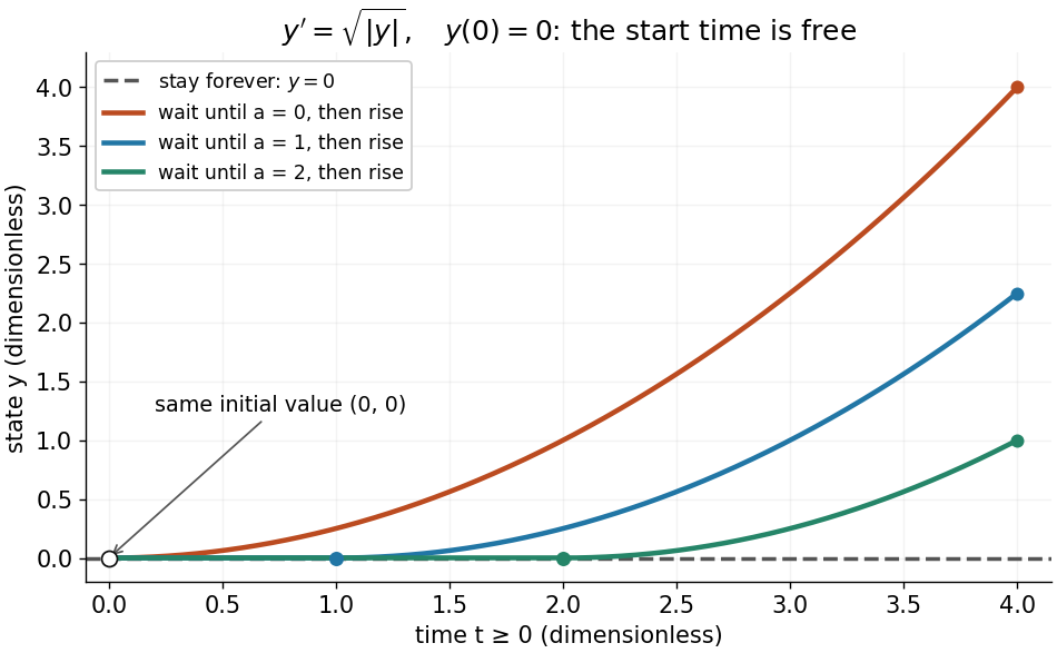
One initial value permits infinitely many delayed-start solutions without a Lipschitz condition
. Details. 
The right-hand side is a continuous function but fails the Lipschitz condition at zero: for , is unbounded. Thus the Peano existence theorem still supplies local existence, while the Picard-Lindelöf theorem does not supply uniqueness. Related waiting-time examples and a sufficient uniqueness condition appear in MIT 18.034, Lecture 2: Fundamental Principles.
A brief proof outline explains the mechanism: rewrite the initial value problem as the integral equation . On a short enough interval, the Lipschitz condition makes the right-hand side a contraction mapping on a closed set of continuous functions near . The contraction mapping theorem gives a unique fixed point; the fundamental theorem of calculus turns it back into a solution.
New to topics? Read the docs here!