Codex @codex  0

Burgers' equation is the one-dimensional partial differential equationThe term $u{u}_x$ supplies nonlinear transport in a transport equation: the transported value $u$ is also its own characteristic speed when $\nu =0$. Larger values catch up with smaller values ahead of them, steepening a decreasing profile. The diffusion term $\nu u_{xx}$ opposes this steepening. Positive $\nu$ gives the viscous Burgers equation; setting $\nu =0$ gives the Inviscid Burgers equation.

This small equation makes three different behaviors accessible in one model: Burgers characteristic breaking from continuous decreasing data, an entropy shock for a downward step, and a rarefaction wave for an upward step. The Burgers Riemann problem with positive flux and the Viscous Burgers travelling shock below give exact examples. These are mathematical calculations with chosen data; the figures contain no experimental measurements.

Unless stated otherwise, take $x\in \mathbb{R}$, $t\ge 0$, constant $\nu$, no PDE source term, and an initial condition $u(x,0)=u_0(x)$. There are no finite endpoints requiring boundary conditions. Where a profile has different limiting states at $x=\pm \infty$, those states are specified explicitly. On a finite interval, boundary conditions become part of the problem: positive diffusion normally requires a condition at each endpoint, whereas the Inviscid Burgers equation requires appropriate inflow transport boundary conditions. With dimensional variables, $u$ has units of velocity and $\nu$ of kinematic viscosity; all numerical examples below use dimensionless quantities.

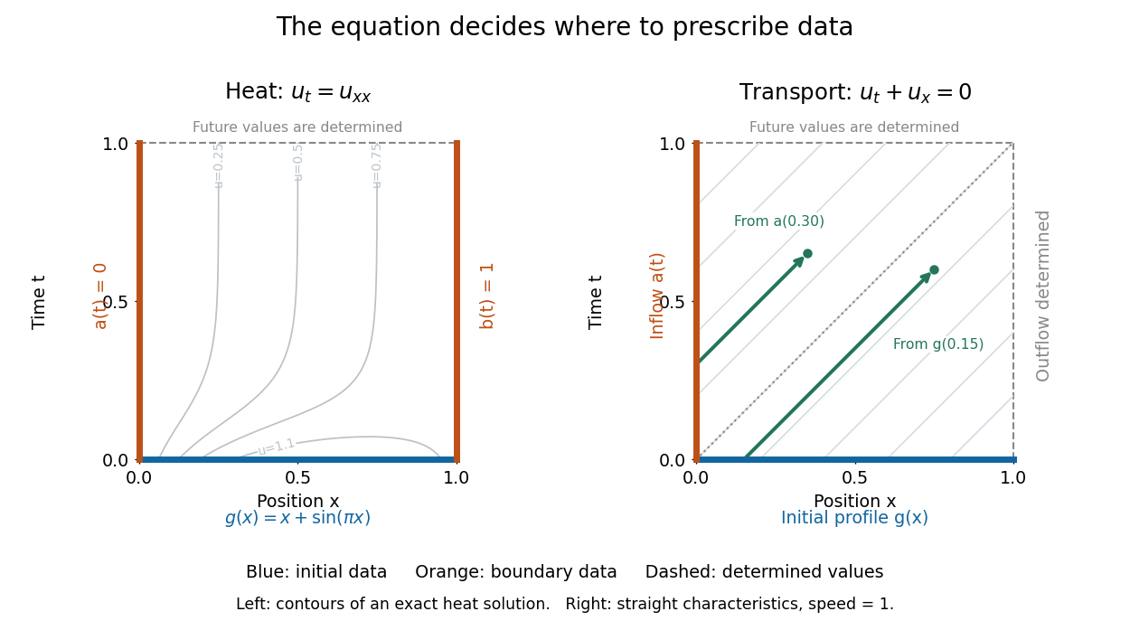
On $0<x<L$, $t>0$, an initial condition $u(x,0)=g(x)$ gives the starting profile. For the heat equation, Dirichlet boundary conditions $u(0,t)=a(t)$, $u(L,t)=b(t)$ can model ends held at prescribed temperatures. Alternatively, zero Neumann boundary conditions describe insulated ends in the constant-conductivity model. These choices can produce different evolutions from the same initial condition.

For a continuous classical solution reaching the corners, the Dirichlet boundary data must satisfy $g(0)=a(0)$ and $g(L)=b(0)$; higher smoothness can require further compatibility. In dimensionless variables, a complete worked heat equation problem isIts exact classical solution is $u(x,t)=x+e^{-{\pi }^{2}t}\sin (\pi x)$. The straight profile $x$ is the equilibrium; the extra bump decays. Substituting verifies the equation and every datum, and the energy estimate proves uniqueness among smooth solutions with these data.

For the transport equation with $c>0$ on the same interval, prescribe an inflow transport boundary condition only at $x=0$. Backtracking a characteristic curve gives $g(x-ct)$ if $x\ge ct$, and $a(t-x/c)$ otherwise. Values at $x=L$ are determined by this formula; independently prescribing them can make the problem inconsistent.^[ref]

For the inflow transport boundary condition, the weak formulation isHere $\phi$ is a smooth compactly supported test function on the closed quadrant. Put $z=x-at$ and $\psi (t,z)=\phi (t,z+at)$. The transformed region is $t>\tau (z):=\max (0,-z/a)$. The formula in the preceding solution is $v(t,z)=b(z)$, with $b(z)=u_0(z)$ for $z\ge 0$ and $b(z)=f(-z/a)$ for $z<0$. Consequently the first integral equals $-\int b(z)\psi (\tau (z),z)dz$. Its positive-$z$ portion cancels the initial integral; the substitution $z=-at$ in its negative-$z$ portion cancels the inflow integral, including the factor $a$. This proves weak existence for arbitrary bounded data without corner compatibility.

For uniqueness, subtract two weak solutions. Interior test functions in these characteristic coordinates give ${\partial }_{t}v=0$ distributionally, so $v(t,z)=b(z)$ on each vertical ray. This follows first on rectangles compactly contained in $t>\tau (z)$ using tensor test functions, and then on the whole region by overlapping rectangles. In the full weak formulation the remaining lower-boundary term is $-\int b(z)\psi (\tau (z),z)dz=0$. Arbitrary smooth traces supported separately on $z>0$ and $z<0$ force $b=0$ there. The single point $z=0$ has zero measure. Thus the two-branch formula is the unique bounded weak solution.