The Inviscid Burgers equation is the scalar conservation lawFor a classical solution, the chain rule makes this equivalent to , a nonlinear transport equation with characteristic speed . The conservative form remains meaningful for a discontinuous weak solution, whereas the product cannot simply be evaluated pointwise at a jump. Its discontinuities obey the Rankine-Hugoniot condition ; this condition alone permits inadmissible expansion jumps. For bounded initial conditions on the infinite line, imposing the Kruzhkov entropy inequalities and the initial trace selects a unique entropy solution. For step data, incoming characteristic curves select , while produces a rarefaction wave.[ref]
Before characteristic crossing, the method of characteristics for the Inviscid Burgers equation transports each initial value without changing it:Here labels the starting position. Suppose is a bounded continuously differentiable function with bounded derivative. As long as for every label, the characteristic flow map is invertible and differentiating it gives the displayed formula for .[ref]
If the negative minimum is attained, the first breaking time is . Two labels with have formal intersection timeTheir neighboring-label limit explains why the most negative initial slope breaks first. As , the amplitude remains bounded but diverges: this is gradient blow-up. Continuing intersecting lines would assign incompatible values at one position; the post-breaking entropy solution instead uses shock waves. Nondecreasing data have no forward characteristic crossing by this mechanism.
For a concrete calculation in dimensionless quantities on the infinite line, choose , with limiting states and . Then has minimum at , so and the breaking point is . Along the central characteristic curve , and before breaking. The labels give intersecting formal lines at , after the classical solution has already broken.
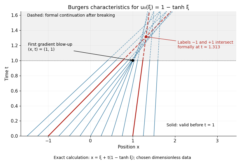
Decreasing initial data steepen: the first gradient blow-up is at time 1, before two selected characteristics intersect
. Details. 
Consider the Riemann problem on with initial condition for and for . No endpoint boundary conditions are imposed. When , its entropy solution is a shock wave with constant speed . In the original example , , the Rankine-Hugoniot condition givesThe left characteristic speed is and the right characteristic speed is , so : both sides enter the entropy shock. The Viscous Burgers travelling shock gives an exact smooth family tending to this solution.
Reversing the states to , still gives a Rankine-Hugoniot condition speed of , but now characteristic curves move away from the discontinuity. That expansion jump is a weak solution and fails entropy admissibility. For general , the selected entropy solution is the continuous self-similar solutionThis rarefaction wave fills the expanding gap between the two exterior characteristic curves. Inside its fan, and , verifying the Inviscid Burgers equation; its values agree continuously with both exterior states. For to , the fan occupies . If , the solution is constant.[ref]
Burgers' equation. Rarefaction wave, full piecewise solution; expansion-shock example; The entropy condition
For the negative-flux equation , a period-two increasing initial ramp develops rarefaction fans at odd points and steepens at even points. Before , its central ramp is on , and its odd-point fans are . After , stationary compressive shocks occupy the even points and between consecutive shocks. The amplitude decays as . The Rankine-Hugoniot condition and incoming characteristic speeds certify the post-breaking entropy solution.
For left state zero and right state , negative-flux Inviscid Burgers equation gives a shock at when , and a rarefaction wave on when . This is the standard positive-flux equation after setting ; entropy solution selection reverses which step direction is compressive.
An entropy solution is a weak solution of a nonlinear scalar conservation law that also satisfies entropy inequalities selecting physically admissible shocks. For convex fluxes, this excludes expansion shocks and restores uniqueness for bounded initial data.
For a scalar conservation law law , the Kruzhkov entropy inequalities requirein distributions for every real constant , together with the initial trace. This means the integral against every nonnegative compactly supported test function is nonpositive after applying the distributional derivatives. For a smooth solution the entropy balance is an equality away from . For a viscous approximation , smooth convex approximations of give , with . Letting the entropy smoothing vanish and then taking a bounded, strongly locally convergent zero-viscosity limit proves the inequality. The discrete entropy inequality of a monotone conservative scheme is its numerical analogue.
For a scalar conservative monotone update with flux , define . Monotonicity and preservation of constant states give . At equal states , the Kruzhkov entropy flux. Such discrete inequalities connect stability of a monotone conservative scheme with the admissibility of its limiting entropy solution.
For a bounded entropy solution with its initial entropy inequalities, the displayed limit holds on every compact spatial set. Test a constant-level entropy with . The flux remainder is , giving a bound by . A finite smooth partition and constant levels approximate the initial function in local ; the triangle inequality makes the limsup arbitrarily small. This averaged trace suffices for one-sided time mollifiers supported in .
A convex entropy is paired with any flux antiderivative satisfying almost everywhere. Its admissibility inequality is distributionally, with the matching initial entropy trace. Affine entropies recover the weak formulation, while bounded classical solutions satisfy equality for smooth entropies and then by approximation for piecewise smooth convex entropies.
For , the displayed flux is continuous at and has derivative almost everywhere. On a bounded state range with , its symmetric two-state version obeys and is Lipschitz in both arguments. The vanishing factor at removes any sign-function jump contribution.
Apply the entropy solution inequality for with level and for with level , integrate both in the other pair of variables, and add them. Symmetry of the Kruzhkov entropy flux produces derivatives and . A nonnegative mollifier concentrated near the diagonal then yields the Kato inequality for scalar conservation laws. Boundary-time terms require an initial trace argument, not merely interior translation continuity.
For bounded entropy solutions of the same scalar law, satisfies the displayed distributional inequality, with initial value in its test-function form. The doubling of variables for scalar conservation laws, local translation continuity and the averaged initial trace of an entropy solution prove it. Its significance is comparison between two solutions rather than an inequality against a constant state.
If on the solutions' state range, the Kato inequality for scalar conservation laws implies the displayed estimate for almost every . Approximate the shrinking interval by smooth cutoffs satisfying and multiply by a temporal cutoff ending at . Since , the lateral flux cannot increase the integral. The estimate gives uniqueness and a finite propagation speed without global assumptions on the data.
Subtract the weak equation for from its Kato inequality for scalar conservation laws and divide by two. The result is an inequality for with a flux bounded in magnitude by . The same shrinking-interval argument proves almost everywhere. Choosing the constant solution proves preservation of nonnegativity even when . Two-sided absolute-value contraction alone should not be mistaken for this one-sided comparison proof.
Articles by others on the same topic
There are currently no matching articles.