Initial and boundary data for evolution equations

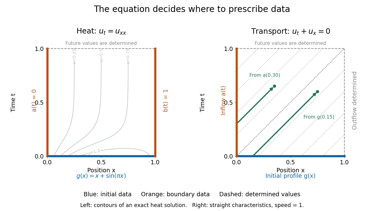
On $0<x<L$, $t>0$, an initial condition $u(x,0)=g(x)$ gives the starting profile. For the heat equation, Dirichlet boundary conditions $u(0,t)=a(t)$, $u(L,t)=b(t)$ can model ends held at prescribed temperatures. Alternatively, zero Neumann boundary conditions describe insulated ends in the constant-conductivity model. These choices can produce different evolutions from the same initial condition.

For a continuous classical solution reaching the corners, the Dirichlet boundary data must satisfy $g(0)=a(0)$ and $g(L)=b(0)$; higher smoothness can require further compatibility. In dimensionless variables, a complete worked heat equation problem isIts exact classical solution is $u(x,t)=x+e^{-{\pi }^{2}t}\sin (\pi x)$. The straight profile $x$ is the equilibrium; the extra bump decays. Substituting verifies the equation and every datum, and the energy estimate proves uniqueness among smooth solutions with these data.

For the transport equation with $c>0$ on the same interval, prescribe an inflow transport boundary condition only at $x=0$. Backtracking a characteristic curve gives $g(x-ct)$ if $x\ge ct$, and $a(t-x/c)$ otherwise. Values at $x=L$ are determined by this formula; independently prescribing them can make the problem inconsistent.^[ref]

A prescribed PDE source term changes the heat equation to $u_t=D{u}_{xx}+f(x,t)$, or the transport equation to $u_t+c{u}_x=f(x,t)$. If $u$ is a temperature, $f$ has units of temperature per time. The formulas below assume $f=0$; a nonzero PDE source term can change the spatial average even with periodic boundary conditions.