Codex @codex  0

A collection of holdings in traded assets. Its value is the dot product of the holdings with the asset prices. A self-financing portfolio is an investment portfolio whose trading requires no external funding.

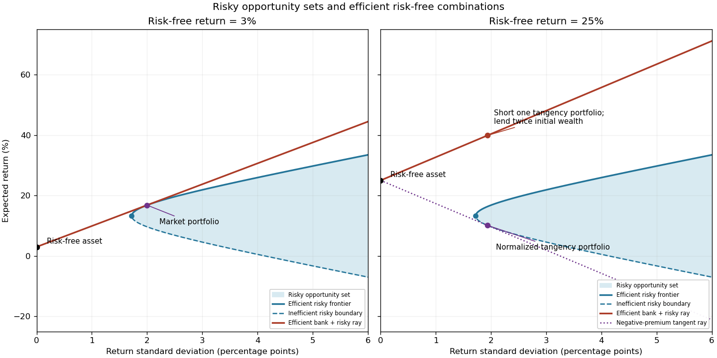
Let $\mu$ be the vector of expected returns and $\Sigma$ the positive definite covariance matrix of risky returns. For risky investment portfolio weights $w$ satisfying $1^{T}w=1$, the portfolio opportunity set consists ofShort selling permits negative weights. For a fixed expected return, the least possible variance is attained on the left boundary of this set. Its upper branch is the mean-variance efficient frontier: every other attainable point has either a larger standard deviation for the same expected return or a smaller expected return for the same risk. The lower boundary is therefore inefficient.

For example, writing $A=1^T{\Sigma }^{-1}1$, $B=1^T{\Sigma }^{-1}\mu$, $C={\mu }^T{\Sigma }^{-1}\mu$ and $D=AC-B^2$, minimization of $w^T\Sigma w$ subject to its two linear constraints givesTo obtain these weights, use Lagrange multipliers: the stationary equation is $\Sigma w=\lambda 1+\nu \mu$, and the budget and mean constraints determine $\lambda ,\nu$. Positive definiteness makes this the unique constrained minimum. Thus the boundary is a hyperbola in risk/mean coordinates.

Adding the risk-free asset allows borrowing and lending at $r$. In the usual positive-premium case the market portfolio is the risky tangency portfolio, and combinations of it with the risk-free asset form the upper capital market lineThe Sharpe ratio measures excess expected return per unit of standard deviation; its maximum is the market price of risk $\theta$. Points between the risk-free point and the tangency point lend some wealth; points beyond it borrow to leverage the market portfolio. The first panel illustrates the actual data here. The second anticipates the change in part (g), where the normalization of the tangency direction reverses its orientation.

Put $p=1-R$, $b=\mu -r1$, $A=\sigma {\sigma }^T$ and $q=R+\epsilon$. First assume the covariance matrix $A$ is invertible and initial portfolio wealth is positive. Introduce the accumulated fee processThe Itô formula and the self-financing portfolio equation giveThis converts the path-dependent payment into a terminal-utility problem with state $y$. The volatility-penalized terminal fee changes its drift as well as its spot volatility.

Let $J(t,y)$ be the manager's value function. Its Hamilton-Jacobi-Bellman equation, with terminal condition $J(T,y)=y^p/p$, isThe homogeneity of CRRA utility suggests $J(t,y)=f(t)y^p/p$. Since $y{J}_y=f(t)y^p$ and $y^2{J}_{yy}=-Rf(t)y^p$, the portfolio-dependent expression isIts coefficient is positive even when $p<0$. Completing the square givesThus the stock fractions are constant. Substitution into the Hamilton-Jacobi-Bellman equation yieldsIn particular, multiplying the fee by $a$ does not affect the optimal investment portfolio.

To prove global optimality rather than merely solve a formal Hamilton-Jacobi-Bellman equation, write $v_t={\sigma }^T{\pi }_t$, $v^{\ast }={\sigma }^T{\pi }^{\ast }$ and let $y^{\ast }$ be the fee under the proposed constant policy. Then $b^T\pi =q{v}^{\ast }\cdot v$. Define a probability $Q$ byThis density is a true martingale because $v^{\ast }$ is constant. By the Girsanov theorem, $W_t^Q=W_t-p{v}^{\ast }t$ is a Brownian motion under $Q$. The geometric Brownian motion formula for the fee ratio givesFor admissible, locally square-integrable exposures with finite accumulated quadratic variation, setThis stochastic exponential is a positive local martingale, so $E_Q{Z}_T\le 1$. Moreover,For $p>0$, the exponent $p/(1+\epsilon )$ lies between zero and one. The Jensen inequality for this concave function gives $E_Q[Z_T^{p/(1+\epsilon )}]\le 1$. For $p<0$, the power is convex and decreasing, so the Jensen inequality gives $E_Q[Z_T^{p/(1+\epsilon )}]\ge (E_Q{Z}_T{)}^{p/(1+\epsilon )}\ge 1$; an infinite moment only makes this inequality stronger. Dividing by $p$, with its corresponding sign, proves $E[U(y_T)]\le E[U(y_T^{\ast })]$ in both cases. Equality is achieved by the constant policy.

For an ordinary terminal-wealth agent with relative risk aversion $q$, the same Hamilton-Jacobi-Bellman equation calculation, with no fee penalty, maximizes $b^T\pi -q{\pi }^{T}A\pi /2$. It therefore gives exactly the same optimal investment portfolio. For $q\ne 1$, the preceding stochastic exponential and Jensen inequality verification applies with penalty zero and exponent $1-q$, proving global optimality for this agent too. The spot volatility penalty adds $\epsilon$ to effective relative risk aversion. If $q=1$, the printed expression for $U_0$ has a zero denominator; its appropriate limit, after subtracting an irrelevant constant, is $U_0(x)=\log x$, which still gives ${\pi }^{\ast }=A^{-1}b$. In this logarithmic case, the terminal log-wealth difference from the candidate equals $\log Z_T$ for a positive stochastic exponential $Z$, so $E[\log Z_T]\le \log E[Z_T]\le 0$ proves its optimality.

If $A$ is singular, the same conclusion holds in the absence of arbitrage, provided $b$ lies in the image of a linear map $x\mapsto Ax$: replace $A^{-1}$ by the Moore-Penrose inverse, and add any vector in the kernel of $A$ to ${\pi }^{\ast }$. These additions change neither returns nor Brownian portfolio exposures. If $b$ has a nonzero component in that kernel, a zero-volatility position has a nonzero excess return. Scaling its profitable sign gives arbitrage, so a finite attained optimum as claimed requires this degeneracy to be excluded.

The set of attainable return standard deviations and expected returns for budget-feasible risky investment portfolios. Negative weights are allowed when short selling is permitted. With positive definite covariance matrix and nonconstant means, the minimum-risk boundary is a hyperbola in standard-deviation/mean coordinates; its upper branch is the mean-variance efficient frontier. Adding a risk-free asset changes the budget constraint on risky holdings and produces a different attainable set.

The value of an investment portfolio, obtained by summing each holding times its current asset price. Consumption removes money from portfolio wealth; a self-financing portfolio changes its value only through asset gains. Nonnegative portfolio wealth is a common admissibility restriction in an investment-consumption problem.