Codex @codex  0

Independence of random variables factors the joint probability mass function as $\mathbb{P}(X=x,Y=y)=\mathbb{P}(X=x)\mathbb{P}(Y=y)$. ThereforeWith finite expected values, these rearrangements are justified by absolute convergence: the analogous sum with absolute values equals $\mathbb{E}[|f(X)|]\mathbb{E}[|g(Y)|]<\infty$. Thus

This numbered item specifies the model used below. A convenient sample space is the collection of $36$ ordered pairs $(s_1,s_2)\in \{1,\dots ,6{\}}^2$, each with probability $1/36$. The corresponding random variables are determined by the sum and difference. Inverting the two equations givesThus a candidate pair $(X,Y)=(i,j)$ is possible exactly when $(i+j)/2$ and $(i-j)/2$ are both integers between $1$ and $6$. In particular, $i$ and $j$ must have the same parity. This inverse description will determine the joint probability mass function.

The independent random variables have a product joint probability mass function. For integers $r,t\ge 0$,It is zero for all other pairs. The factors are the respective Poisson distribution masses, with the product justified by independence.

Summing the two nonzero entries with $X=1$ givesThe remaining probability is $\mathbb{P}(X=0)=1-p$, so $X$ has the Bernoulli distribution with parameter $p$.

For the other marginal, the two entries at $Y=0$ add to $e^{-p}$, the entry at $Y=1$ is $p{e}^{-p}$, and for $k⩾2$ the only nonzero entry is already $e^{-p}{p}^k/k!$. Thusand $Y$ has the Poisson distribution with parameter $p$. This also checks normalization of the joint probability mass function by summing the marginal.

There is no such value of $p$ in the specified interval. Indeed, $\mathbb{P}(Y=1)=p{e}^{-p}>0$, and the joint probability mass function givesThis contradicts independence for every $0<p<0.8$. Equivalently, $(1,2)$ has joint probability zero but the product of its marginal probabilities is $p{e}^{-p}{p}^2/2>0$.

At the suggested value $r=e^{-r}$, the covariance is zero, but the same conditional probability contradiction still applies. This is an explicit example of how uncorrelated Bernoulli and Poisson variables need not be independent. Zero covariance controls one mixed moment, whereas independence requires the entire joint probability mass function to factor.

The joint probability mass function is $p_{X,Y}(x,y)=\mathbb{P}(X=x,Y=y)$ for $(x,y)\in S^2$. It is nonnegative and its sum over $S^2$ equals one. Summing over one coordinate gives the other variable's marginal distribution.

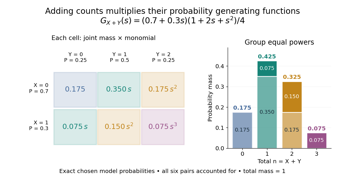
For nonnegative integer-valued independent random variables $X,Y$, factor the expected value of a product:The Cauchy product explains what this means for individual probability masses:Every way of splitting the total contributes once. This is convolution of independent random variables; multiplying probability generating functions performs the bookkeeping automatically.

For an original example, take independent $X\sim \mathrm{Bernoulli}(0.3)$ and $Y\sim \mathrm{Binomial}(2,0.5)$, using the Bernoulli distribution and binomial distribution. ThensoDirect enumeration of the six pairs $(x,y)$ gives the same probability masses. For example, total one collects $(0,1)$ and $(1,0)$, with contributions $0.7\cdot 0.5+0.3\cdot 0.25=0.425$. The coefficients sum to one. The expected value is $G_{X+Y}^{\prime }(1)=1.3$; since $G_{X+Y}^{\prime \prime }(1)=1.1$, the variance is $1.1+1.3-1.3^2=0.71$, agreeing with $0.3\cdot 0.7+2\cdot 0.5\cdot 0.5$.

Uncorrelated random variables are insufficient for the product identity. For a concrete counterexample, let $U$ be uniform on $\{-1,0,1\}$ and set $A=U+1$, $B=U^2$. Then $\mathrm{Cov}(A,B)=\mathbb{E}[U^3]=0$, but $\mathbb{P}(A+B=0)=0$, whereas $G_A(0)G_B(0)=1/9$. Zero covariance controls one mixed moment, not the full joint probability mass function.