The sample space is the set of outcomes represented by a probability model. One elementary outcome specifies a complete result at the level of detail the model keeps. An event is a subset belonging to the model's sigma-algebra ; it occurs when the actual outcome lies in that subset. Together with a probability measure , these form a probability space , with .[ref]
Introduction to Probability, Statistics, and Random Processes by Hossein Pishro-Nik. §1.3.1 Random Experiments: definitions of outcome, sample space, and event; three-toss example
Choosing a sample space means deciding which distinctions matter. For two tosses, recording the ordered head-or-tail sequence distinguishes from ; recording only the number of heads merges them. Neither representation is automatically wrong, but the second cannot answer a question about which toss was heads. Keeping a detailed sample space and defining a random variable for the desired observation lets several questions share one model.
A sample space alone assigns no probabilities. Even writing as a Cartesian product does not establish independence: that requires a condition on the probability measure. On a finite sample space with all subsets admitted as events,Only when all elementary probabilities are equal does this become , where the bars denote cardinality. This is the uniform distribution on a finite set, an additional modelling choice.
Sample spaces can also be infinite. For example, take , its Borel sigma-algebra, and the continuous uniform distribution. Then for , so each singleton has probability zero while . Thus an elementary outcome need not carry positive probability, and a continuous model cannot be understood by counting equally likely points. The distinction is developed in zero-probability event and countable additivity.
A family of disjoint events whose union is the sample space. For the countable law of total probability and law of total expectation, use a finite or countably infinite family. Conditioning formulas sum only positive-probability parts, or interpret zero-probability contributions as zero without assigning a conditional expectation there.
An elementary outcome is one member of the sample space. For the ordered two-toss model, is one outcome; it contains both toss results. By contrast, “at least one head” is an event containing three outcomes. The outcome and the singleton set are different objects: when that singleton is measurable, the notation gives its probability. In the finite model below, every subset is measurable.
The word elementary refers to the chosen level of detail. An outcome can be an ordered pair, a sequence, or an entire realization of a point process. A random variable then extracts a numerical feature of that outcome; the window count of a point process is one example.
Model two fair independent coin tosses, recording their order. Here denotes heads and tails, andThe power set includes every question expressible as a subset of these four outcomes. The mass comes from the fairness and independence assumptions. These are exact model probabilities, rather than measured toss frequencies.
Let be the event that the first toss is heads and the event that the second toss is heads. ThenThe union means “at least one head,” while the intersection means “both heads.” Their probabilities are and . Counting the union through the inclusion-exclusion principle gives ; alternatively its complement of an event is , of probability .
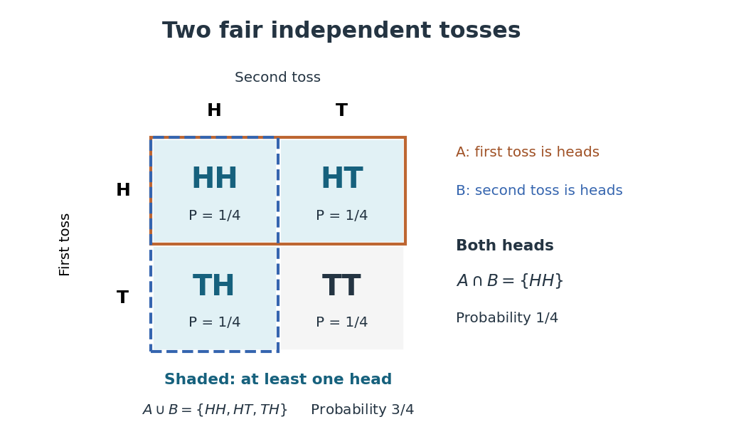
Four ordered outcomes and the event of at least one head
. Rows record the first toss and columns the second. Each cell has probability under fair independent tosses. The highlighted union includes , , and ; the overlap contains only . Details.On the same sample space, assigning masses to would still make each toss fair: . But , so the tosses would be dependent. The event of at least one head would have probability . Changing the probability measure changes the answer even when the sample space and the single-toss probabilities stay the same.
Define the head-count random variable byThe four elementary outcomes are inputs to this function; its three numerical values are outputs. Each fiber of a function collects all outcomes giving one value. Under the fair independent model, adding the masses in each fiber gives the probability mass functionConsequently the output values are not equally likely, although the inputs are. Using the reduced sample space with these masses gives the same head-count probability distribution; assigning to each value would describe a different model.
A question about a random variable's value becomes an event on the original sample space by taking an inverse image:For a real-valued random variable, this is an event whenever is a Borel set, by measurability. In this finite example every subset of is allowed. In particular,This is the same “at least one head” event counted above, expressed through an observable.[ref]
Random: Probability, Mathematical Statistics, Stochastic Processes by Kyle Siegrist. Probability Spaces, §2 Events and Random Variables, Random Variables: measurable functions and the inverse-image notation for value events
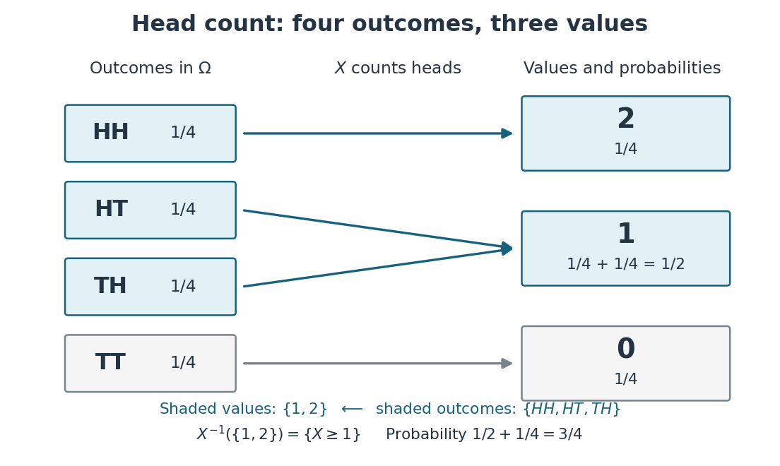
Head count merges outcomes into fibers and adds their probabilities
. The random variable sends to zero, both and to one, and to two. The inverse image of is the highlighted event of at least one head. Two arrows meeting at one explain its probability . Details.Every event determined by is a union of complete fibers. There are such events, whereas the full power set of has . In particular, the first-head event is not determined by : it contains but excludes , although both give . Choosing an observable makes calculations simpler precisely by forgetting distinctions; the useful choice is one that retains the distinctions the question needs.


