Kernel trick

The kernel trick evaluates inner products of feature map outputs through $k(x,z)=⟨\varphi (x),\varphi (z)⟩$ without explicitly constructing those vectors. An algorithm expressed entirely through these inner products can therefore operate on nonlinear derived coordinates using only evaluations of a positive-semidefinite kernel on the original inputs. A classifier linear in the derived coordinates can have a nonlinear boundary in the original coordinates.

The polynomial kernel gives a finite, fully visible example: $k(x,z)=(x^{T}z{)}^2$ corresponds to $\varphi (x)=(x_1^2,\sqrt{2}{x}_1{x}_2,x_2^2{)}^T$. The XOR separation by a product feature below makes the interaction coordinate $x_1{x}_2$ useful, while dual prediction with a kernel shows how to predict without calculating it explicitly.

An arbitrary score called a similarity need not be a positive-semidefinite kernel. Symmetry alone, even with nonnegative entries, is insufficient: the symmetric matrixhas $a^{T}Sa=-2$ for $a=(1,-1{)}^T$, so it cannot be a Gram matrix of real inner products. A positive-semidefinite kernel requires a positive semidefinite matrix for every finite choice of inputs, not just the observed training data.^[ref] The existing Moore-Aronszajn theorem connects this requirement to a Reproducing kernel Hilbert space; this example needs only finite linear algebra.

Give the four corners of the square the exclusive or labels: $+1$ when the input signs differ and $-1$ when they agree. In the following order,No affine function $g(x)=a_1{x}_1+a_2{x}_2+b$ has the required strictly positive scores at $p_2,p_3$ and strictly negative scores at $p_1,p_4$: both pairs have midpoint zero, so $g(p_2)+g(p_3)=2b=g(p_1)+g(p_4)$ would have to be both positive and negative. This also rules out perfect classification by a single threshold with a consistent tie rule.

Under the polynomial kernel's quadratic feature map, the two classes become two distinct vectors:The hyperplane ${\varphi }_2=0$ separates them. With $w=(0,-1/\sqrt{2},0{)}^T$ and $b=0$, the score and classifier areAll four signed scores $y_{i}f(p_i)$ equal one. In the input plane the boundary is $x_1{x}_2=0$, the union of the coordinate axes; in the derived coordinates it is a single hyperplane. The feature map identifies opposite corners, which is harmless for these labels because opposite corners belong to the same class. A fixed feature map would not separate labels that disagree at identical mapped vectors.

If the weight vector lies in the linear span of the training feature map outputs, write $w={\sum }_i{\beta }_i\varphi (p_i)$. ThenThis is a dual representation: coefficients weight training examples rather than feature coordinates. They need not be positive, and need not be unique when the kernel matrix is singular. 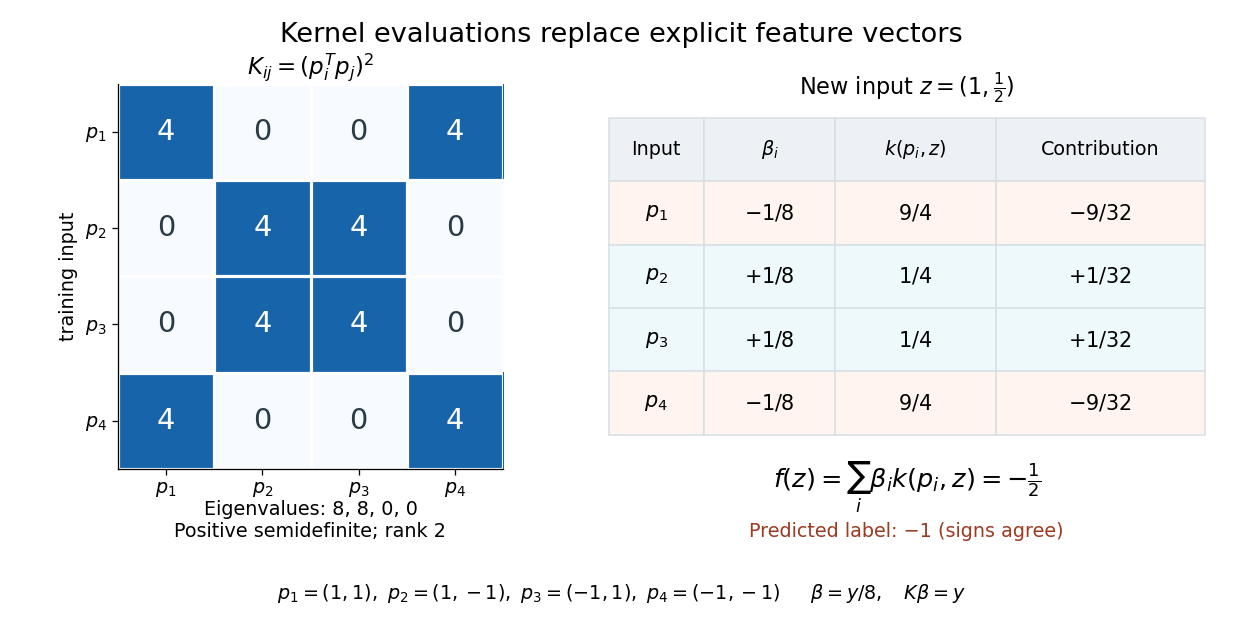Some kernel methods instead write ${\beta }_i={\alpha }_i{y}_i$ with ${\alpha }_i\ge 0$ under their own optimization constraints.^[ref] The formula is an algebraic conversion for a weight vector in this linear span, not a claim about every possible weight vector. The representer theorem gives a broader reason this form appears in regularized kernel methods.

For the XOR separation by a product feature, let $\Phi$ have rows $\varphi (p_i{)}^T$. The Gram matrix of those rows, equivalently the kernel matrix, isIts eigenvalues are $8,8,0,0$, so it is a positive semidefinite matrix of rank two, not an invertible matrix. More generally, for any real coefficient vector $a$ and any finite set of inputs,This proves the positive-semidefinite kernel condition for the displayed polynomial kernel on all of ${\mathbb{R}}^2$, rather than checking only this square.

Here $Ky=8y$, so the explicit choice $\beta =y/8$ gives $K\beta =y$ and ${\Phi }^T\beta =w$. ConsequentlyFor the new input $z=(1,1/2)$, the four polynomial kernel evaluations are $(9/4,1/4,1/4,9/4{)}^T$. Their weighted sum is $-1/2$, and the sign function predicts $-1$. No explicit feature map is needed for this calculation. These coefficients were constructed to reproduce the chosen separator; no fitting algorithm or generalization guarantee is being asserted.

For $d$ input coordinates, the homogeneous quadratic polynomial kernel has a weighted quadratic feature map with $D=d(d+1)/2$ distinct monomials. Computing an inner product of already stored mapped vectors costs $O(D)$ arithmetic operations, whereas $(x^{T}z{)}^2$ costs $O(d)$ using the input vectors. Here $O$ denotes big O notation. Higher fixed degrees can make the dimension gap much larger.

Sample count still matters. With $n$ training examples, materializing a dense kernel matrix stores $n^2$ numbers and requires $n(n+1)/2$ distinct evaluations using symmetry. A dense direct solve for kernel ridge regression typically takes $O(n^3)$ operations after constructing the kernel matrix, while a dual prediction with $m$ nonzero coefficients uses $m$ kernel evaluations. Explicit finite feature maps can be preferable when $D$ is small relative to $n$, and a stored primal weight vector can make prediction depend on $D$ rather than on $n$. The kernel trick by Ryan Giordano (sections Ridge regression and The polynomial kernel) explains the change from feature-coordinate equations to training-example equations; neither representation is universally faster.

The kernel trick saves explicit feature construction when the positive-semidefinite kernel is economical to evaluate; it does not remove the cost of optimization, choose a useful positive-semidefinite kernel, or establish generalization. Random Fourier features illustrate a different tradeoff: replacing the exact Gaussian kernel with a finite approximate feature map can reduce dependence on the sample count while introducing approximation error.

Kernel principal component analysis diagonalizes a centered kernel matrix to perform principal component analysis in an implicit feature space.