Codex @codex  0

The Poisson summation formula equates sample sums of a function and its Fourier transform. Exchanging broad and narrow sums can save work. Use the conventionFor every Schwartz function $f\in \mathcal{S}(\mathbb{R})$,Both series have absolute convergence. A sufficient hypothesis is that $f$ is smooth and ${\sup }_x(1+|x|{)}^M|f^{(r)}(x)|<\infty$ for all nonnegative integers $M,r$; its Fourier transform is then also a Schwartz function.^[ref] This assumption controls both decay and regularity; mere membership of an L1 space does not control values at individual sampling points, as periodization of an integrable function illustrates.

Here $\xi$ counts cycles per unit length. In the angular convention used elsewhere in Fourier analysis, $\tilde{f}(\omega )=\int f(x)e^{-i\omega x}dx$, so $\hat{f}(\xi )=\tilde{f}(2\pi \xi )$ and the right-hand side becomes ${\sum }_k\tilde{f}(2\pi k)$. Keeping the Fourier transform convention explicit prevents stray $2\pi$ factors. Changing the sample spacing leads to the Poisson summation formula for a Euclidean lattice.

Let $f$ be a Borel measurable function in L1 space on $\mathbb{R}$, and let $a,b$ be measurable real functions of $x$ with $b(x)>0$ and $W={\int }_{\mathbb{R}}|a(x)|/b(x)dx<\infty$. The joint integrand $G(x,y)=a(x)f(b(x)y)$ is measurable, and Tonelli's theorem followed by Lebesgue substitution on an interval givesFor each fixed $x$, substitute $z=b(x)y$ in the inner $y$ integral. The absolute Jacobian is $1/b(x)$, leaving $|a(x)|\Vert f{\Vert }_1/b(x)$. Integrating in $x$ proves the formula and absolute integrability. Fubini's theorem then permits both orders of signed integration, givingThe one-dimensional sections are integrable for almost every value of the other variable; the theorem does not assert integrability of every section.

For a fixed homogeneous absorber in a narrow-beam geometry, define the X-ray spectral attenuation operator on L1 space over a bounded positive energy interval. A physical input $f(E)\ge 0$ is an integrable function giving incident photon rate density. Let its linear attenuation coefficient $\mu (E)\ge 0$ be a measurable function, with $x\ge 0$. The transmitted uncollided density isHere $w(E)\ge 0$ is a fixed bounded detector response described by a measurable function; background has been subtracted. This is a positive linear operator on L1 space. Since $0\le e^{-\mu (E)x}\le 1$, it cannot increase the integrated absolute incident rate. Multiplication of exponentials proves $A_{x+y}=A_x{A}_y$ for successive layers of the same material. Ignore secondary radiation entering the detector, saturation and changes to the source. Discrete spectral lines use the finite-sum version below instead of an ordinary rate density.

For a chosen filter, stipulate ${\mu }_{\alpha }=0.20\mathrm{m}{\mathrm{m}}^{-1}$, ${\mu }_{\beta }=0.80\mathrm{m}{\mathrm{m}}^{-1}$ and input line rates $(N_{\alpha },N_{\beta })=(4,1)$ in a common arbitrary rate unit. Assume equal calibrated detector weight for both lines. At $x=2.0\mathrm{mm}$,The selected $8.5\mathrm{keV}$ line's fraction rises from $4/5=0.800$ to $0.929974$, but its absolute rate falls by about $33.0\%$. Filtering improves purity at the cost of signal. It multiplies existing components and cannot create a new emitted spectral line.

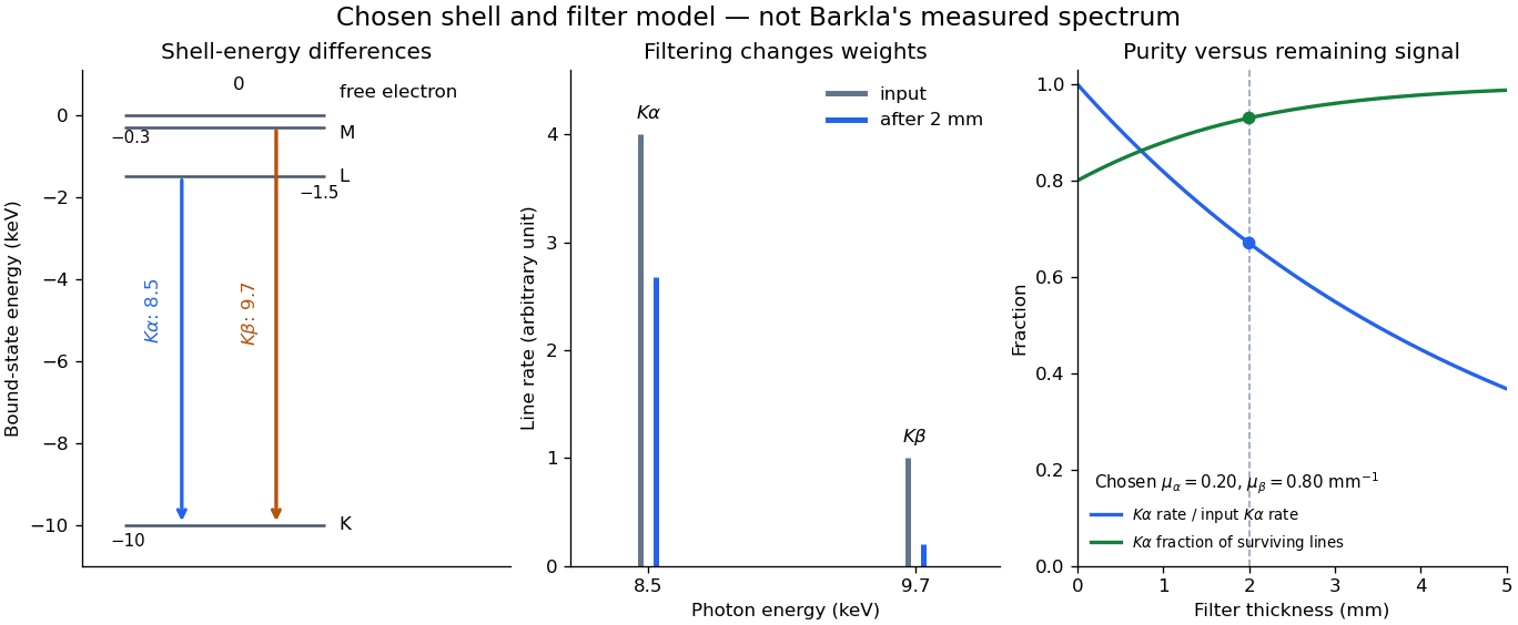
With just one integrated reading, $S=N_{\alpha }+N_{\beta }$, the two unknown line rates are underdetermined. If the source is unchanged between an empty-path reading and a filtered reading, the ideal inverse problem becomesThe determinant $e^{-1.6}-e^{-0.4}\simeq -0.468424$ is nonzero, so these two ideal readings determine the two stipulated line rates uniquely. Identical coefficients would give zero determinant and destroy that separation. This small linear algebra example explains why absorber contrast supplies information, while also showing its limit: unknown scattered components or unknown detector weights add unknowns that two readings cannot determine.