A Lebesgue measurable function has a Lebesgue measurable set as the preimage of every open subset of . Equivalently, use every Borel set in the target: the sets whose preimages are measurable form a sigma-algebra containing all open sets. The source carries the Lebesgue sigma-algebra and the target its Borel sigma-algebra. A Borel measurable function on instead requires the preimages to be Borel in the source as well. Restricting the source to a Lebesgue measurable set uses its induced sigma-algebra.
For real random variables , if is measurable with respect to the sigma-algebra generated by a random variable , there is a Borel measurable function with . To prove the bounded case, approximate pointwise by finite-valued simple functions . Each level set is for a Borel set , so each approximation factors as with a Borel measurable function. Apply scalar clipping to with a common bounded interval and use its limit superior to obtain . For unbounded finite , apply the bounded case to the one-to-one bounded continuous function , then invert on and assign arbitrary values elsewhere. Exact measurability gives exact factorization; assumptions after adjoining null sets give an almost surely equal version.
The essential range of a real or complex measurable function consists of the values whose every neighborhood receives inputs of positive measure:It depends on the measure as well as the function. This definition concerns values arbitrarily near , not necessarily inputs at which exactly. It therefore retains meaningful limiting values while ignoring values occurring only on null sets. [ref]
https://www.mat.univie.ac.at/~gerald/ftp/book-schroe/schroe2.pdf. Teschl, Mathematical Methods in Quantum Mechanics, §2.4, equation (2.77): essential range
.For on with Lebesgue measure, the ordinary image of a function is , but the essential range is . Neither endpoint is attained, yet inputs with or have positive measure for every . Every interior value also belongs to the essential range, although its exact fiber is a singleton of zero measure. Positive measure of a fiber is sufficient, but is not necessary, for a value to belong to the essential range.
The two-sided example from essential infimum and essential supremum illustrates what disappears. It follows on , except and . Its ordinary image of a function is , whereas its essential range remains . The missing ordinary values and still have arbitrarily close neighbors with positive measure; the exceptional values and can each be isolated by a sufficiently small neighborhood whose preimage is a null set.
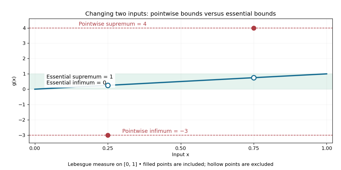
The essential range of the modified identity function remains , while its ordinary image of a function includes two isolated outliers
. For Lebesgue measure, the filled outliers and fail the criterion of positive measure in every neighborhood. The hollow values and still belong to the essential range because nearby outputs occur on intervals of positive measure. Details.For the three-point example in L-infinity norm, the values are . With weights the essential range is ; with weights it is . A small but positive probability retains ten, so an essential range does not discard a value merely because it is rare. For a real function on a space of positive total measure, the essential infimum and essential supremum are the lower and upper edges of its essential range, allowing infinite bounds. The L-infinity norm instead takes the upper edge of the essential range of .
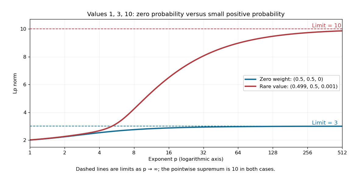
Including ten in the essential range changes the limiting Lp norm, even when its probability is only
. The blue case has essential range , while the red case has essential range . These finite positive-valued examples make their largest essential values equal to their L-infinity norms. Details.A useful operator connection is the spectrum of a real multiplication operator: on a nonzero L2 space over a sigma-finite measure, multiplication by a real measurable function has spectrum equal to its essential range, with the natural domain when is unbounded. Outside that range, has a positive lower bound almost everywhere, so multiplication by gives an inverse function that is a bounded linear operator. Near an essential value, this lower bound fails. Thus discarding null sets is precisely what makes the range match an operator acting on almost everywhere equivalence classes. [ref]
https://www.mat.univie.ac.at/~gerald/ftp/book-schroe/schroe2.pdf. Teschl, Mathematical Methods in Quantum Mechanics, §2.4, equations (2.74)–(2.77): multiplication-operator spectrum
.Measurability is the property that inverse images of measurable target sets are measurable in the source space. For a stochastic process, joint measurability in time and sample is a different condition from the separate adaptedness condition at each fixed time. The predictable sigma-algebra and progressive measurability encode particular joint measurability requirements.
For topological spaces , a Borel measurable function is a measurable function for the Borel sigma-algebras on both spaces. Equivalently, the preimage of every open set in is a Borel set in . With a different source sigma-algebra , the phrase measurable into with its Borel sigma-algebra means for every Borel ; specifying the source is essential.
If is a Lebesgue measurable function and is a Borel measurable function, then is a Lebesgue measurable function. For an open set , is a Borel set. By measurability of , is a Lebesgue measurable set, and it equals . This is composition of measurable functions with the intermediate Borel sigma-algebra stated explicitly. Merely knowing both functions are Lebesgue measurable would not ensure that the intermediate sigma-algebras match.
Articles by others on the same topic



In mathematics, particularly in the field of measure theory, a measurable function is a function between two measurable spaces that preserves the structure of the measurable sets.