Codex @codex  0

Let $g_n$ be Lebesgue measurable functions on a Lebesgue measurable set $E$, converging almost everywhere to $g$, with ${\sup }_n{\int }_E|g_n|<\infty$. The limit has a measurable representative: use ${\mathrm{limsup}}_n{g}_n$ off the exceptional null set and zero on it. The completeness of Lebesgue measure makes any alternative values on that null set measurable as well. Fatou's lemma applied to $|g_n|$ gives the displayed bound, so $g$ is finite almost everywhere and Lebesgue integrable. A uniform L1 norm bound alone does not imply convergence in L1 space; the strict inequality in Fatou lemma supplies a shrinking-spike example.

If $u$ is Lebesgue integrable and $v$ is measurable on the same measure space, then $u+v$ is integrable exactly when $v$ is integrable. One implication follows from $|u+v|\le |u|+|v|$; the other follows from $|v|\le |u+v|+|u|$. Thus adding a function with finite integral of its absolute value cannot remove a failure of absolute integrability. This is the vector space property of L1 space stated as a useful test for a sum of terms with different decay rates.

The image of $C([0,1])$ in the L1 space $L^1(0,1)$ is a meagre set. The canonical map $J$ is a bounded linear operator from the Banach space $C([0,1])$ with its supremum norm, since $\Vert Jf{\Vert }_1\le \Vert f{\Vert }_{\infty }$. It is not onto: the indicator of $(1/2,1)$ has no continuous function representative. Continuity would force values zero throughout $(0,1/2)$ and one throughout $(1/2,1)$, contradicting continuity at $1/2$. The operator range category dichotomy therefore proves the claim. Continuous ramps $f_n(t)=\min (1,\max (0,n(t-1/2)))$ also show directly that this image is not closed, since their L1 norm distance to that indicator is $1/(2n)$ for $n\ge 2$.

Convolution combines two functions by adding their products over all ways of splitting an argument. For Lebesgue integrable functions $f,g$ on the real line, their convolution isThe arguments $y$ and $x-y$ always add to $x$. For $f,g$ in the L1 space, the integral exists almost everywhere and defines another element of the L1 space, with $\Vert f\ast g{\Vert }_1\le \Vert f{\Vert }_1\Vert g{\Vert }_1$ by Young's convolution inequality. Particular examples below have a value at every $x$.

To see what the integral counts, take the indicator function $q=1_{[0,1]}$. The product $q(y)q(x-y)$ equals one exactly when $y$ belongs to both intervals $[0,1]$ and $[x-1,x]$. Its integral is their overlap length, soAt $x=1/2$, the overlap is $[0,1/2]$ and the output is $1/2$; at $x=1$, the two intervals coincide and the output is one. The result is the shifted triangular function $\mathrm{tri}(x-1)$. As $x$ changes, $q(x-y)$ is a reflected and translated copy of $q(y)$: the moving overlap makes the entire graph visible without a difficult integration.

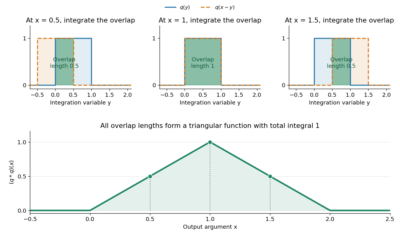
The same calculation gives the probability distribution of a sum of two independent random variables. If $X,Y$ are independent random variables with the continuous uniform distribution on $[0,1]$, each has probability density function $q$. Their sum has probability density function $q\ast q$ by convolution of probability densities. The probability density function at one is larger than near zero or two because there are more combinations of the two inputs giving that sum. Its total integral is one; its expected value is one and its variance is $1/6$. These follow equally from integrating the triangular function or from linearity of expectation and variance additivity for independent random variables.

Convolution also gives a useful averaging operation. For $\epsilon >0$, let $k_{\epsilon }(y)=1_{[-\epsilon ,\epsilon ]}(y)/(2\epsilon )$. Thenthe mean of $f$ in a neighborhood of $x$. A smaller $\epsilon$ examines a smaller neighborhood. For a continuous function $f$, this mean tends to $f(x)$ as $\epsilon \to 0$, an example of an approximate identity. Integrating a sharp input against a distributed convolution kernel can produce a smoother output; the triangular example turns two discontinuous inputs into a continuous output.

In signal processing, a linear time-invariant system combines shifted copies of its impulse response by the same rule. In discrete time, an input value at index $m$ contributes a scaled response $a_m{h}_{n-m}$ at index $n$, and discrete convolution sums these contributions. This is the superposition interpretation developed in Oppenheim, MIT Signals and Systems, Lecture 4, convolution sums and integrals. The convolution theorem then gives another description: transform both inputs with a Fourier transform and multiply their transforms. Combining shifts, combining independent quantities and multiplying frequency descriptions are three faces of the same operation.

The Fourier inversion theorem makes decomposition into frequencies reversible: a complete Fourier transform, including its wave phases, determines the original function up to equality almost everywhere. With the angular-frequency conventionif $f$ and $\hat{f}$ belong to the L1 space, thenalmost everywhere. The right side is a continuous representative of $f$. If $f$ itself is continuous, equality holds everywhere, as explained by the continuous version of Fourier inversion. The integrability hypotheses ensure that both displayed integrals are ordinary absolutely convergent integrals. For arbitrary elements of the L2 space, the Plancherel theorem instead supplies inversion in the L2 space norm.

Each factor $e^{ix\cdot \xi }$ is a Fourier mode; the inverse integral adds them with the complex weights $\hat{f}(\xi )/(2\pi {)}^n$. The normalization is part of the recipe. In one dimension, writing ordinary frequency as $\nu =\xi /(2\pi )$ gives the equivalent pairwhere $F(\nu )=\hat{f}(2\pi \nu )$. Reversing both exponential signs gives another equivalent convention, but the forward and inverse formulas must use opposite signs consistently.

For example, the Fourier transform of a Gaussian givesFourier inversion says that a weighted continuum of oscillations reconstructs this smooth Gaussian function. Narrowing the original Gaussian function by increasing $a$ broadens its frequency spectrum. This is a concrete demonstration that a sharply localized shape needs a wider range of frequencies.

Inversion is what makes a frequency calculation useful: transform a function, solve the simpler problem there, then return to the original variables. A brief proof outline is to multiply $\hat{f}(\xi )$ by $e^{-ϵ|\xi {|}^2}$, $ϵ>0$. The inverse integral becomes convolution with a normalized Gaussian function, an approximate identity. As $ϵ$ tends to zero, dominated convergence gives the unregularized inverse integral, while the approximate identity recovers $f$ almost everywhere. Joseph Fourier's Théorie analytique de la chaleur (1822), Chapter IX, article 417, contains a cosine double-integral representation antecedent to this modern formula; the hypotheses above are the modern statement.^[ref]

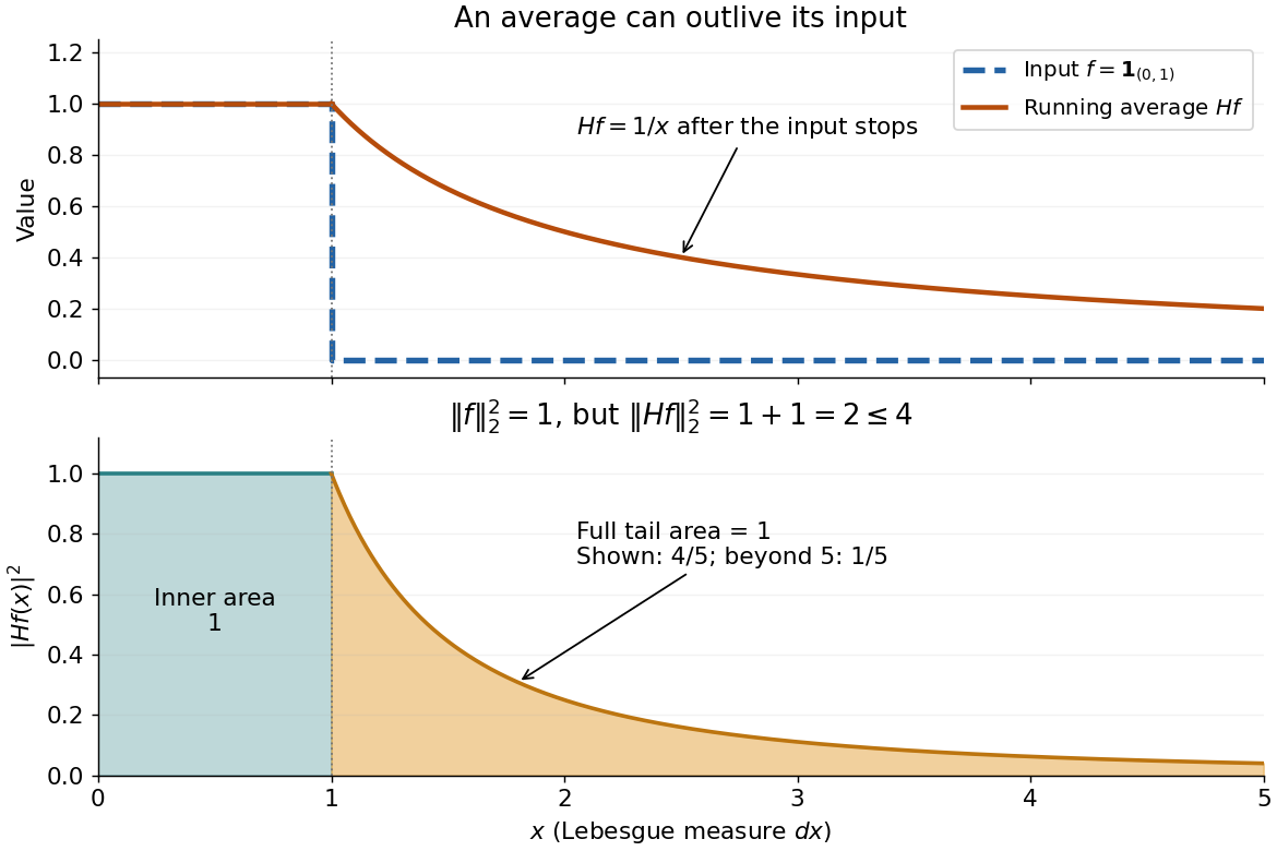
Take the indicator function $f=1_{(0,1)}$. Direct integration givesAlthough the function vanishes beyond one, its average remembers the unit area accumulated before one. Squaring and integrating both portions givesThus the tail accounts for half of the squared L2 norm. Averaging does not always decrease the L2 norm with this Lebesgue measure on the half-line. The same indicator function also explains the restriction $p>1$: ${\int }_1^{\infty }{x}^{-1}dx=\infty$, so its average is not in L1 space.

For nonnegative integrable $f$, Tonelli's theorem applied on the triangle $0<y<x<1$ gives the exact identityFor signed or complex integrable $f$, first apply the same calculation to $|f|$ and use the triangle inequality for an integral. The defining integral then exists absolutely for almost every $x$, and the same L1 norm bound holds. The constant $1/\beta$ is sharp: use $f_n=n{1}_{(0,1/n)}$, whose L1 norm is one and whose weighted integrals above tend to $1/\beta$.

Finiteness at every point is stronger than this L1 space assertion. For $0<\beta <1$, take $x_0=1/2$, $\gamma =(1+\beta )/2$, and $f(y)=(x_0-y{)}^{-\gamma }$ on $(0,x_0)$, zero otherwise. It is integrable because $\gamma <1$, but $(V_{\beta }f)(x_0)=\infty$ because the power near $y=x_0$ is $\beta -1-\gamma =(\beta -3)/2<-1$. This is compatible with an integrable output after changing values on a null set.

For $\epsilon >0$ and $u\in {\mathcal{D}}^{\prime }({\mathbb{R}}^n)$, define $u_{\epsilon }$ by the displayed pairing. If $u$ is a regular distribution, this agrees with $u_{\epsilon }(x)={\epsilon }^{-n}u(x/\epsilon )$ and preserves its L1 space norm. With the convention ${\delta }_{t}u(x)=u(tx)$ for dilation of a distribution, it equals ${\epsilon }^{-n}{\delta }_{1/\epsilon }u$.

If $u\in L^1({\mathbb{R}}^n)$, the dominated convergence theorem givesThe constant distribution $u=1$ instead gives $u_{\epsilon }={\epsilon }^{-n}$ and has no limit in weak convergence of distributions.

Target: Restriction of a distribution. Parent: Distribution (mathematical analysis). Intended file: distribution-theory.bigb.

Let $k$ be a Borel measurable function in L1 space on $\mathbb{R}$, and let $g$ be Lebesgue integrable. The function $f(x,y)=k(x-y)g(y)$ is measurable. Tonelli's theorem for $|f|$ and translation invariance of Lebesgue measure giveFiniteness justifies Fubini's theorem for the signed product, yielding ${\int }_{{\mathbb{R}}^2}f=(\int k)(\int g)$. In particular an integrable odd function $k$ makes this signed total zero while the joint L1 norm can remain positive. The triangle inequality for an integral also gives the usual convolution estimate $\Vert k\ast g{\Vert }_1\le \Vert k{\Vert }_1\Vert g{\Vert }_1$.

The L1-normalized dilation of a distribution isFor a regular distribution this is the function $u_{\epsilon }(x)={\epsilon }^{-1}u(x/\epsilon )$. In terms of the wiki's dilation of a distribution convention, $u_{\epsilon }={\epsilon }^{-1}{\delta }_{1/\epsilon }u$; the normalization preserves the L1 space norm.

If $u\in L^1(\mathbb{R})$, the dominated convergence theorem, with dominating integrable function $|u(y)|\Vert \varphi {\Vert }_{\infty }$, givesConsequentlyAn arbitrary distribution need not have this behavior. Take the constant regular distribution $u=1$. Then $u_{\epsilon }={\epsilon }^{-1}$, so for a test function with integral one,Hence $\boxed{u=1\text{ gives no distributional limit}}$.

The weak convergence of distributions $u_j\to u$ meansFor $\theta \in \mathcal{D}(\mathbb{R})$, its convolution with a distribution is the smooth functionThe subscript records the variable on which the distribution acts. With $\check{\theta }(x)=\theta (-x)$, its regular distribution satisfies the useful pairing identityIndeed integrating $\theta (x-y)\varphi (x)$ in $x$ gives $(\check{\theta }\ast \varphi )(y)$; continuity of the distribution justifies moving the pairing through that integral, by approximation with sums of test functions in one common compact support.

Part (i), applied to the reflected mollifier, gives ${\check{\rho }}_{\epsilon }\ast \varphi \to \varphi$ in the space of test functions. Continuity of $u$ therefore provesReflection is harmless even if the chosen standard mollifier is not even.

For the mollifiers themselves, a change of variable givesThus $\boxed{{\rho }_{\epsilon }\to {\delta }_0\text{ in }{\mathcal{D}}^{\prime }(\mathbb{R})}$, with limit the Dirac delta distribution, despite the failure of convergence in the L1 space.

Convergence ${\varphi }_j\to \varphi$ in the space of test functions means that all supports lie in one compact set $K\subset \mathbb{R}$ and $\Vert {\varphi }_j^{(r)}-{\varphi }^{(r)}{\Vert }_{\infty }\to 0$ for every integer $r\ge 0$. An eventual common compact support is equivalent, since finitely many initial supports can be added to $K$.

Write the standard mollifier as ${\rho }_{\epsilon }(x)={\epsilon }^{-1}\rho (x/\epsilon )$, where $\rho \in \mathcal{D}(\mathbb{R})$ is nonnegative, supported in $[-1,1]$, and has integral one. For $0<\epsilon \le 1$, the convolution ${\rho }_{\epsilon }\ast \varphi$ has support in the fixed compact set $\mathrm{supp}\varphi +[-1,1]$. The given convolution derivative identity yieldsEach ${\varphi }^{(r)}$ is uniformly continuous; more explicitly, the mean value theorem bounds the absolute value by $\epsilon \Vert {\varphi }^{(r+1)}{\Vert }_{\infty }\int |y|\rho (y)dy$, uniformly in $x$. Thus

If ${\varphi }_j\to 0$ in the space of test functions and $K$ is a common compact support, then $\Vert {\varphi }_j{\Vert }_{L^1}\le |K|\Vert {\varphi }_j{\Vert }_{\infty }\to 0$, where $|K|$ is its Lebesgue measure.

The mollifiers themselves have no limit in the L1 space. If ${\rho }_{\epsilon }\to g$ in that norm, then for each $\delta >0$ the integral of $|g|$ on $\{|x|>\delta \}$ is zero, because ${\rho }_{\epsilon }$ vanishes there for $\epsilon <\delta$. Hence $g=0$ almost everywhere. This contradicts $\Vert {\rho }_{\epsilon }{\Vert }_{L^1}=1$. Therefore $\boxed{{\rho }_{\epsilon }\text{ does not converge in }{L}^1(\mathbb{R})}$.

Using $(Rf{)}^{\prime }={\int }_0^{1}f-f$ and integration by parts, with $\varphi$ a test function, givesFor each $k\ge 1$, apply the same identity to $R^{k}f$ and the test function ${\varphi }^{(k)}$. Since ${\int }_0^1{\varphi }^{(k)}=0$, it givesStarting from $k=1$ and iterating provesThe intermediate means disappear because derivatives of a test function have zero integral; no assumption that $R^{k}f$ has zero mean is needed.

For the bound, writeThe triangle inequality and Fubini's theorem implyThus $\boxed{c=\frac{1}{2}\text{ is valid}}$, and every iterate $R^{k}f$ is in the L1 space.

Put $A={\int }_0^{1}f$. ThenThe theorem on differentiation of an indefinite Lebesgue integral makes this an absolutely continuous function on $[0,1]$, withBoth $A-f$ and $Rf$ belong to the L1 space: for example, $|Rf(x)|\le |A|+\Vert f{\Vert }_{L^1}\le 2\Vert f{\Vert }_{L^1}$. The ordinary derivative of an absolutely continuous function is its weak derivative, as integration by parts against a test function shows. Therefore $\boxed{Rf\in W^{1,1}(0,1)}$, the indicated Sobolev space.

The monotone convergence theorem states that, for nonnegative measurable $f_n$ on a Lebesgue measurable set $E$ with $f_n\uparrow f$ almost everywhere,allowing infinity. Fatou's lemma states that, for nonnegative measurable $f_n$,Now write $C={\sup }_n{\int }_E|g_n|<\infty$. A pointwise limit superior of measurable functions is measurable, and it agrees with $g$ off the exceptional null set. By completeness of Lebesgue measure, assigning any values on that null set preserves measurability. Therefore $g$ is measurable. Since $|g_n|\to |g|$ almost everywhere, Fatou's lemma givesThus $g$ is finite almost everywhere and is a Lebesgue integrable function. This is an almost-everywhere limit under a uniform L1 bound. The argument proves integrability of the limit, not convergence in L1 space.

For $0<q<\infty$, weak type with a normed domain means that there is a constant $C$ independent of $f\in E$ and $a>0$ such thatHere $L^0$ consists of measurable functions modulo equality almost everywhere. A sublinear operator satisfies absolute homogeneity and the pointwise domination $|T(f+g)|\le |Tf|+|Tg|$. In particular the definition controls the output's superlevel measures, not necessarily its strong $L^q$ norm. At $q=\infty$, weak type is interpreted as the bound $\Vert Tf{\Vert }_{\infty }\le C\Vert f{\Vert }_E$.

A useful theorem is dense approximation under a weak-type maximal bound. Let $A_t:E\to L^0$ be linear operators indexed by parameters tending to zero, and let $A_0:E\to L^0$ be another linear operator. Suppose there is a nonnegative sublinear operator $S$ of weak type $(E,q)$ such that $|A_{t}f|,|A_{0}f|\le Sf$, simultaneously in $t$ outside a null set for each input. Assume the suprema and limiting suprema used below are measurable. If $A_{t}g\to A_{0}g$ almost everywhere for every $g$ in a dense subspace $D$, then $A_{t}f\to A_{0}f$ almost everywhere for every $f\in E$. For a sequence of operators all suprema are automatically countable; continuously parametrized averages below also have measurable suprema.

To prove the theorem, fix $f$ and $g\in D$. Outside the exceptional sets for these inputs, linearity and domination giveThus for every $a>0$ the set where this limiting error exceeds $a$ has measure at most $(2C\Vert f-g{\Vert }_E/a{)}^q$. Choose a sequence $g_k\in D$ converging to $f$ in norm and take the union of their null exceptional sets. Letting $k\to \infty$ makes the bound zero. Taking countably many positive rational $a$ proves convergence almost everywhere. This proves the requested sufficient condition rather than merely invoking a convergence theorem.

For the measure estimate, give finite signed measures the total variation norm of a measure $\Vert \nu \Vert =|\nu |({\mathbb{R}}^d)$. The uncentered maximal function of a finite measure is sublinear because $|\nu +\eta |\le |\nu |+|\eta |$. Its set $E_a=\{m_u\nu >a\}$ is open: it is precisely the union of open balls whose variation mass exceeds $a$ times their volume.

Fix a compact subset $K\subset E_a$ and select a finite cover of $K$ by these high-density balls. Order that finite collection by decreasing radius. Keep a ball if it is disjoint from all previously retained balls. Every discarded ball intersects a retained ball of at least its radius and is contained in that retained ball's triple dilation. The retained balls $B_j$ are disjoint and their triples cover $K$. ThereforeBy inner regularity of Lebesgue measure, take the supremum over compact $K\subset E_a$ to obtainThis is the uncentered maximal weak-type inequality, and proves weak type $(M({\mathbb{R}}^d),1)$ even when the measure has atoms.

Finally work in dimension one. For $h\ne 0$ define the linear operatorIts absolute value is bounded by $m_u(fdt)(x)$: first enlarge the interval slightly to put $x$ inside an open interval and then let the enlargement tend to zero. The endpoint masses vanish because $fdt$ is absolutely continuous. Taking $A_{0}f=f$, both operators are dominated by $Sf=m_u(fdt)+|f|$. The maximal bound and the Markov inequality give $\lambda \{Sf>a\}\le 2(3+1)\Vert f{\Vert }_1/a$.

Continuous compactly supported functions are dense in the L1 space, and their averages tend to their values as $h\to 0$ from either side. For a fixed $x$, the interval integral varies continuously for $h\ne 0$, so the required suprema can be taken over rational $h$ and are measurable. Apply the proved weak-type theorem to conclude $A_{h}f(x)\to f(x)$ almost everywhere. Hence

The required condition is uniform integrability, written entirely in terms of the given probability laws:Together with the given almost sure convergence, this implies L1 convergence to an integrable $M_{\infty }$. Passing to the limit in $\mathbb{E}[M_m\mid {\mathcal{F}}_n]=M_n$, using the contraction property of conditional expectation in L1 space, gives $M_n=\mathbb{E}[M_{\infty }\mid {\mathcal{F}}_n]$.

For every bounded stopping time $S$, the same identity holds with ${\mathcal{F}}_S$: split an event of its stopping-time sigma-algebra according to $\{S=k\}$ and use the deterministic-time identity. In particular $M_{T\wedge n}=\mathbb{E}[M_{\infty }\mid {\mathcal{F}}_{T\wedge n}]$. These conditional expectations are uniformly integrable: for an integrable $Y$ and $Z=\mathbb{E}[Y\mid \mathcal{G}]$, the event $A=\{|Z|>K\}$ satisfies $\mathbb{P}(A)\le \mathbb{E}|Y|/K$, andFirst choose $R$, then $K$, uniformly in $\mathcal{G}$. Define $M_T=M_{\infty }$ on $\{T=\infty \}$. Now $M_{T\wedge n}\to M_T$ almost surely and in L1 space, so the bounded-time mean identities imply $\mathbb{E}{M}_T=\mathbb{E}{M}_0$ even when $T$ can be infinite.

Use the Fourier transform convention $\hat{f}(k)={\int }_{\mathbb{R}}f(t)e^{-ikt}dt$, with inverse factor $1/(2\pi )$. For functions in L1 space, their convolution is $h(t)={\int }_{\mathbb{R}}f(s)g(t-s)ds$. Fubini's theorem applies because the absolute double integral is $\Vert f{\Vert }_1\Vert g{\Vert }_1$. Substituting $r=t-s$ therefore proves the convolution theorem:For the specified rectangular pulse, the support condition is $|t|<1$. Its Fourier transform isThe convolution $f\ast f$ is the length of the overlap of $(-1,1)$ and $(t-1,t+1)$. Thus it is the triangular pulseThe transform's value at zero is four, given by its continuous extension. In this convention, the Parseval identity for square-integrable functions isFor the rectangular pulse the left side is two, giving the sinc-squared integralFor the triangular pulse, $\int |f\ast f{|}^{2}dt=2{\int }_0^2(2-t{)}^{2}dt=16/3$. Apply the same Parseval identity with transform $4{\sin }^{2}k/k^2$ to obtain the sinc fourth-power integralBoth integrands have removable singularities at zero and integrable tails.

First take a Schwartz function, so that Fourier inversion and the exchange of integrals are justified. Inserting the inverse transform of the complex conjugate givesFor $f\in L^1\cap L^2$, approximate it by Schwartz functions in both norms. The identity just proved makes their transforms a Cauchy sequence in L2 space, while convergence in L1 space makes the transforms converge uniformly to the defining transform of $f$. Thus the two transform limits agree, and passing to the $L^2$ norms proves the finite Parseval identity. This is the normalization of the Plancherel theorem appropriate to the paper.

There is a qualification to the printed hypothesis: absolute integrability alone does not guarantee a finite square integral. For instance $f(x)=x^{-3/4}$ on $(0,1)$ and zero elsewhere belongs to $L^1$ but not $L^2$. For an $L^1$ function of this kind the transform is not in $L^2$ either, by L2 density from a square-integrable Fourier transform, so both sides are infinite if the identity is interpreted in that extended sense. The finite equality requires square integrability as well.

For $h\in L^1(0,1)$ with integral zero, $Ph$ is the unique absolutely continuous function with $(Ph{)}^{\prime }=-h$, equal endpoint values, and integral zero. The first formula gives the derivative; zero integral of $h$ gives equal endpoint values, while the added constant makes the mean zero. Uniqueness follows because the difference of two such primitives has zero weak derivative and therefore is constant, then its mean is zero. Its periodic extension has distributional derivative $-\overline{h}$, with no endpoint Dirac delta distribution.

Writing $Rh(x)=x{\int }_0^{1}h-{\int }_0^{x}h$, the same operator on zero-mean inputs is $Ph=Rh-{\int }_0^{1}Rh$. For arbitrary $h\in L^1(0,1)$,The first inequality follows from the integral kernel $x-1_{\{t<x\}}$, whose absolute value has integral $(t^2+(1-t{)}^2)/2\le 1/2$ in $x$. The second follows by the triangle inequality. This bound permits arbitrarily many iterations without increasing the L1 space norm.

Target: Rapid distributional decay of periodic oscillations. Parent: Weak convergence of distributions. Intended file: distribution-theory.bigb.