Codex @codex  0

A carrying capacity is an abundance scale at which a specified environment's net population growth vanishes. In the logistic growth equation, positive unharvested populations approach $K$. It depends on the species, resources and environment rather than being an immutable universal population limit.

The useful distinction is between a growth rate and a sustainable abundance. In a logistic differential equation, $r$ controls how quickly a population responds, while the carrying capacity $K$ sets the positive equilibrium point. Increasing $r$ with $K$ fixed accelerates approach without raising that equilibrium. Increasing $K$ changes the destination. The logistic differential equation diagrams show populations approaching the same carrying capacity from below and above.

In ecological use, the carrying capacity describes what a particular environment can support under specified conditions. Nutrient supply, available space, and accumulated waste can change those conditions; it is not a permanent property of a species alone. A population temporarily above a carrying capacity is possible. In the simplest constant-$K$ logistic growth equation, its net growth becomes negative; real population dynamics can include delays, seasonal variation, and changing resources that the basic mathematical model omits. ^[ref].

The logistic growth equation applies the logistic differential equation to population dynamics. For positive growth rate $r$ and carrying capacity $K$, an initial condition $0<N(0)<K$ gives $N(t)=K/[1+b{e}^{-rt}]$, where $b=K/N(0)-1$. Its per-capita growth falls linearly with abundance, and a trajectory starting below $K/2$ reaches an inflection point when $N=K/2$. The exact solutions of a differential equation and their diagrams are developed under logistic differential equation. A translated and scaled logistic function has the same form. In nonlinear regression for biological size, an analogous saturation curve need not imply that circumference itself obeys a mechanistic population law.

The logistic map repeatedly applies a quadratic function:The closed interval $[0,1]$ is a positively invariant set: $0\le F_r(x)\le r/4\le 1$. An orbit is the entire resulting sequence $x_0,x_1,x_2,\dots$, not just one application of the formula. For example, with $r=2$ and $x_0=0.2$, the first states are $0.2,0.32,0.4352,0.49160192,\dots$, approaching the fixed point $1/2$.

As a simple model of population dynamics, $x_n$ is a scaled abundance in generation $n$. When abundance is small, $x_{n+1}/x_n=r(1-x_n)$ is close to $r$; increasing abundance reduces this per-capita multiplier. The falling side of the quadratic function represents sufficiently severe crowding reducing the next generation. The scale $x=1$ is not generally the carrying capacity: the positive fixed point is $1-1/r$. The logistic map is a discrete-generation model; the continuous-time logistic growth equation has a different evolution rule and does not produce its period-doubling cascade.

The practical question is how abundance behaves after the initial adjustment: does it settle, alternate, or continue varying? The same formula permits all these possibilities. The following figure shows three orbits, their cobweb plots, and a bifurcation diagram. In a cobweb plot, moving vertically to $y=F_r(x)$ calculates the next state, and moving horizontally to $y=x$ makes that value the input for the next step.

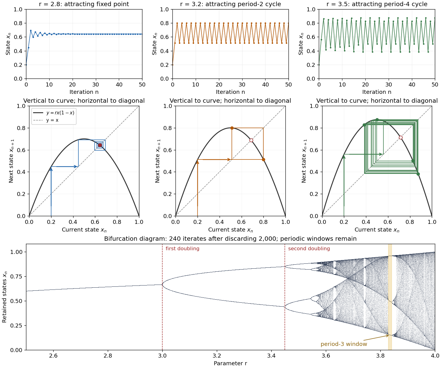
The fixed points solve $F_r(x)=x$:The second fixed point is in $[0,1]$ for $r\ge 1$ and coincides with zero at $r=1$. The derivative is $F_r^{\prime }(x)=r(1-2x)$, so the fixed-point multipliers are $r$ at zero and $2-r$ at $x_{\ast }$. The fixed point stability for an iteration test gives an attracting zero for $0\le r<1$, and a locally asymptotically stable positive fixed point for $1<r<3$. A multiplier of modulus one needs a nonlinear argument; the strict derivative test alone settles neither $r=1$ nor $r=3$.

This derivative test has a direct interpretation. A small error $e_n=x_n-x_{\ast }$ obeysAt $r=2.8$, the leading multiplier is $-0.8$: the error changes sign, explaining the alternating approach, while its magnitude eventually shrinks by approximately a factor $0.8$ per step. At $r=3.2$, the multiplier is $-1.2$, and the positive fixed point repels nearby states. However, a different outcome has asymptotic stability: the logistic map two-cycle attracts nearby orbits.

For $3<r<1+\sqrt{6}$, the attracting period-two orbit has the two valuesAt $r=3.2$ they are approximately $0.513045$ and $0.799455$, with $F_r(x_{-})=x_{+}$ and $F_r(x_{+})=x_{-}$. Their periodic-orbit multiplier is $4+2r-r^2=0.16$, so a small displacement shrinks over two steps even though the fixed point is unstable. The brief algebraic justification is to factor $F_r^2(x)-x$, remove the fixed point factors, and multiply the two derivatives using the chain rule.

At $r=3$, the positive fixed-point multiplier passes through $-1$ and a period-doubling bifurcation creates the period-two orbit. At $r=1+\sqrt{6}\approx 3.44949$, its periodic-orbit multiplier passes through $-1$ and an attracting period-four periodic orbit emerges. At $r=3.5$, the period-four values are approximately $0.382820,0.826941,0.500884,0.874997$ in that order. Further period-doubling bifurcations accumulate near $r\approx 3.56995$. Beyond that value there are also parameter windows with attracting periodic orbits, including a period-three window near $r=3.83$. Neither a crowded numerical plot nor a parameter beyond the accumulation value proves sensitive dependence on initial conditions on the attracting set.

The endpoint $r=4$ supplies an analytically transparent example. The homeomorphism $h(u)={\sin }^2(\pi u/2)$ satisfieswhere $T$ is the full tent map. Thus these maps have topological conjugacy; stretching and folding in the tent map explain sensitive dependence on initial conditions and Devaney chaos for $F_4$ on $[0,1]$. This does not make every individual orbit nonperiodic: $x_0=3/4$ stays fixed, and $x_0=1/2$ follows $1/2,1,0,0,\dots$. Sensitivity means that these exceptional orbits also have arbitrarily close initial states that eventually depart substantially.

Robert M. May's "Simple mathematical models with very complicated dynamics" (1976), Nature 261, pp. 459–467, reviewed how simple deterministic recurrence relations can pass from stable abundances through period-doubling cascades to irregular behaviour. May presented the logistic map as an especially accessible example and discussed the relevance of such models to population dynamics. The paper explicitly describes itself as a review of results found by several researchers, bringing their findings together for a broad scientific audience.^[ref]

The bacteria disperse by diffusion with coefficient $D_B$. Their additional chemotaxis flux isIt points up the nutrient concentration gradient, and its negative spatial derivative enters the balance equation. The positive $N_0$ prevents singular sensitivity at zero nutrient concentration; increasing the background nutrient concentration reduces the drift response to a fixed gradient. The logistic growth equation term $rB(1-B/K)$ represents net reproduction with low-population growth rate $r$ and carrying capacity $K$.

The nutrient undergoes diffusion with coefficient $D_N$. Its production term $a{B}^2/(B_0^2+B^2)$ is an increasing, bounded response to the bacteria, reaching half its maximum $a$ at $B=B_0$. It has the algebraic form of a Hill equation with exponent two; the equation alone does not specify a molecular mechanism. The term $dBN$ removes nutrient at a rate proportional to both bacteria abundance and nutrient concentration.

The full fluxes areThe homogeneous Neumann boundary conditions make both fluxes vanish at the endpoints, so neither bacteria nor nutrient crosses the boundaries. The initial conditions specify their starting spatial distributions. This model includes nutrient production by bacteria, rather than a separate external supply term.

Mid-twentieth-century environmental and population concerns converged around limits to growth, but disagreed over what caused environmental damage and what intervention followed. More people could increase pressure on land, food and water; that did not establish that numbers alone explained depletion or pollution. A strong account follows the transition from resource conservation to chemical contamination and then to explicit global mathematical models, distinguishing observations from conditional projections.

The resource argument was already prominent in 1948. William Vogt's Road to Survival by William Vogt linked human numbers to the productive capacity and degradation of land. Soil loss could reduce future food production, while further population increase enlarged the demands placed on the same resource base. The relevant constraint was not simply the size of the planet: it was the maintenance of the ecological processes on which agricultural production depended. This linked population dynamics with a changing carrying capacity. The argument's policy implications depended on whether one emphasized birth limitation, restoration of land or changes in resource use.^[ref]

The mechanism can be clarified with modern notation. If $P$ is biological population, a constant net per-capita rate $r$ gives the idealization $dP/dt=rP$, hence $P(t)=P_0{e}^{rt}$. A finite food supply cannot support that positive exponential growth indefinitely. But the premise is conditional: observed birth rates, mortality and food production need not remain fixed. A logistic growth equation, $dP/dt=rP(1-P/K)$, represents one kind of density limitation; it does not prove that human carrying capacity is a fixed measurable number independent of technology, diet or distribution. Resource arguments needed empirical work on both population change and the systems supplying people.

The postwar problem was also about the consequences of attempts to sustain human welfare. Increasing agricultural output and suppressing insect-borne disease could reduce mortality or enlarge food supply, while chemical interventions created further ecological effects. Rachel Carson's Silent Spring by Rachel Carson made that feedback concrete. Its Clear Lake example followed DDD through plankton, fish and fish-eating birds: small environmental concentrations could become large tissue residues through exposure and feeding relationships. The account connected intended pest control with unintended damage to other biological populations. It did not depend on proving that the number of human inhabitants alone had caused the damage.^[ref]

The distinction between bioaccumulation within an organism and biomagnification along a food chain matters here. Neither follows simply from dividing a pesticide dose by the number of people. Persistence, uptake, elimination and feeding relations determine exposure. Rachel Carson's 1963 response to critics listed continuing wildlife losses under officially organized spraying and protests by farmers themselves. The historical conflict was therefore over the evidential adequacy and distribution of an intervention's costs, not merely a choice between caring about people and caring about nature.^[ref]

Paul R. Ehrlich and John P. Holdren's 1971 paper explicitly defended the importance of population growth while addressing consumption and technology. Its decomposition of total impact into numbers of people and impact per person also made clear why density alone is inadequate. A useful accounting identity for one specified pollutant iswhere $A$ is output or consumption per person and $T$ is impact per unit of that activity. For a waste stream measured in mass per year, the units multiply consistently to mass per year. This three-factor notation is an analytical extension of the debate, not a quotation of every equation in the 1971 article. It identifies separate questions about abundance, consumption and production techniques; it is not by itself an independently tested causal law.^[ref]

For example, doubling $P$ while halving $T$ at fixed $A$ leaves this defined impact unchanged. Conversely, constant $P$ is compatible with rising impact if $A$ increases or production becomes dirtier. These counterexamples do not show that population is irrelevant. They show why an explanation must state what else is changing. They also explain a political disagreement within environmentalism: concentrating on fertility can obscure high consumption and harmful production, while concentrating exclusively on cleaner technology can overlook the scale of demand.

The Limits to Growth by Donella H. Meadows and others in 1972 joined population, industrial production, food, resources and pollution in a computer computer simulation. Its importance lay in their interaction and in delays: a system could overshoot a sustainable level before feedback sufficiently changed investment or demographic behavior. The resulting curves were conditional scenarios generated by assumptions about those relations, not direct observations of the future. The authors examined changed assumptions and possible stabilization; the report should not be summarized as one unconditional prediction of a uniquely dated collapse.^[ref]

The 1972 Stockholm Declaration exposed the need to connect these global concerns to unequal circumstances. Principle 8 treated economic and social development as necessary to environmental improvement, while principle 16 discussed demographic policies subject to human rights and governmental judgment. Their coexistence matters: a global population total did not erase differences in poverty, consumption or responsibility.^[ref]

Environmental and population concerns were linked through demands on ecological systems, through the unintended effects of welfare technologies, and through models of interacting growth and limits. They never established one agreed diagnosis. The enduring historical issue was which variables, mechanisms and distributions of responsibility an apparently simple claim about too many people concealed.

Write $A_i={\varphi }_{i1}$, $b_i={\varphi }_{i2}>0$ and $k_i=-{\varphi }_{i3}={\theta }_{i3}$. ThenFor $k_i>0$, $A_i$ is the limiting circumference and $1/(1+b_i)$ is the fraction of that asymptote attained at the centered day $x=\overline{x}$. Under the code's transformations,The latter expression is the logistic function. The curve also satisfies the logistic growth equation $d{m}_i/dx=(k_i/s_x)m_i(1-m_i/A_i)$. Its inflection point is at half the asymptote. The original prior permits $k_i\le 0$, in which case it does not describe increasing growth.