Codex @codex  0

Electron optics studies how electric fields and magnetic fields guide Electrons and form images. The Lorentz force supplies a trajectory description, while the de Broglie wavelength supplies the wave scale needed for diffraction. Both descriptions matter: steering a narrow beam and resolving two nearby specimen features are different achievements.

For a magnetic electron lens,Here $e>0$ is the elementary charge, $\mathbf{v}$ the Electron velocity, and $\mathbf{B}$ the magnetic field. The second equality follows because a cross product is perpendicular to each factor: a static magnetic field bends the trajectory without increasing the kinetic energy. Acceleration instead requires work by an electric field. This distinction lets an electron microscope adjust imaging with magnetic fields while an accelerating voltage sets the Electron momentum.

A magnetic electron lens uses a solenoid around the beam axis; iron pole pieces concentrate its magnetic field.^[ref] A strictly axial trajectory in a perfectly uniform axial magnetic field experiences no Lorentz force, since $\mathbf{v}\times \mathbf{B}=0$. Near the entrance, a radial field component turns an advancing Electron azimuthally; the resulting sideways velocity in the axial magnetic field also produces a radial Lorentz force. This couples image rotation and focusing. Real trajectories bend smoothly, whereas a thin lens diagram compresses that bending into one effective plane.

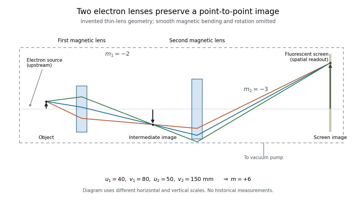
Consider two ideal thin electron lenses in successive imaging stages. In each stage choose positive object and image distances $u_i,v_i$ for a real image, measured from its effective lens plane, and neglect the image rotation of a magnetic electron lens. The paraxial approximation givesThe product follows directly by writing $y_1=m_1{y}_0$ and $y_2=m_2{y}_1$. Here $m_i$ is transverse magnification, rather than the enlargement applied later to a photograph. Both inversions cancel in this planar model; actual magnetic electron lenses can additionally rotate the image.

For an original worked example, take $u_1=40\mathrm{mm}$, $v_1=80\mathrm{mm}$, $u_2=50\mathrm{mm}$ and $v_2=150\mathrm{mm}$. ThenA $100\mu \mathrm{m}$ object interval becomes $600\mu \mathrm{m}$ at the screen. The second lens sits $v_1+u_2=130\mathrm{mm}$ after the first. These are calculated distances, not measurements of the 1931 instrument.

To measure magnification, divide a screen interval between corresponding grid features by the independently known object interval. Repeat over several periods to reduce endpoint uncertainty. For a proposed check, record accelerating voltage, lens electric currents, screen position and specimen orientation; compare one-stage and two-stage images, refocusing as necessary. Changing a lens electric current should change focus and scale, while a blank exposure checks detector background. Keep irradiation and recording enlargement controlled, and repeat the original setting to test drift or specimen damage. These are suggested checks, not a claim that every check was performed in 1931. A grid-scale measurement establishes magnification; resolving much finer features requires a separate target and contrast criterion.