An electron microscope forms a spatially enlarged representation of a specimen using Electrons, electron lenses, and a detector. Its appeal is access to structure too fine for an ordinary optical microscope, but a short de Broglie wavelength alone does not guarantee fine electron microscope resolution. Increasing magnification can enlarge an existing blur without revealing any additional structure.
In transmission electron microscopy, an electron gun illuminates a thin specimen; magnetic electron lenses form and enlarge its transmitted image on a fluorescent screen or detector. A vacuum reduces collisions with gas. Lens electric currents control focusing and magnification.[ref]
Transmission Electron Microscope (TEM) by JEOL. JEOL, The difference between Electron Beam and Light: gun, vacuum, magnetic lenses and screen
Electron microscopy is the practice of preparing specimens, producing images with an electron microscope, and interpreting their contrast. A dark region can reflect Electron deflection out of the admitted beam rather than complete absorption. A useful image therefore needs a stated preparation, detection signal and length calibration; brightness by itself does not identify a material. Transmission electron microscopy probes thin specimens, whereas a scanning electron microscope can examine the exposed surface of a bulk specimen.[ref]
Scanning Electron Microscopes (SEM) by JEOL. JEOL, Observation of the micro world using electrons and Various Function of SEM: transmitted versus surface-generated signals
Transmission electron microscopy images Electrons transmitted through a thin specimen. Electron diffraction from a selected region supplies complementary information about its atomic arrangement. A useful transmitted signal requires suitable specimen thickness.[ref]
Transmission Electron Microscope (TEM) by JEOL. JEOL, Another characteristic electron diffraction: thin specimens, images and diffraction patterns
The image also depends on which outgoing Electron directions reach the detector. Transmission electron microscopy contrast makes this selection explicit: changing the objective aperture can change an image without changing the specimen. Interpreting the result requires electron diffraction, a specified detector response and measurement calibration.
Transmission electron microscopy contrast is a difference in recorded signal between specimen regions under specified illumination, angular acceptance and detector settings. For a positive reference signal , one possible signed contrast convention isNegative means darker than the reference; it does not specify a surface height or chemical composition. The definition must accompany a numerical contrast value, since other conventions exist. A conspicuous feature need not establish fine spatial resolution: detecting a small signal difference and distinguishing two nearby features are different measurement questions.
An objective aperture selects outgoing Electron directions in the objective lens's back focal plane. Passing the central transmitted beam gives bright-field transmission electron microscopy; selecting a separated diffracted beam gives dark-field transmission electron microscopy.[ref]
In a paraxial approximation, an outgoing angle maps approximately to position in this focal plane, where is the objective focal length. A centred opening of radius therefore admits . Selecting a direction selects a component of the outgoing wavefunction; the subsequent image still assigns intensity to specimen positions. The opening is not a hole cut into a real-space specimen image. Its angular selection must be distinguished from selecting a specimen region for electron diffraction.
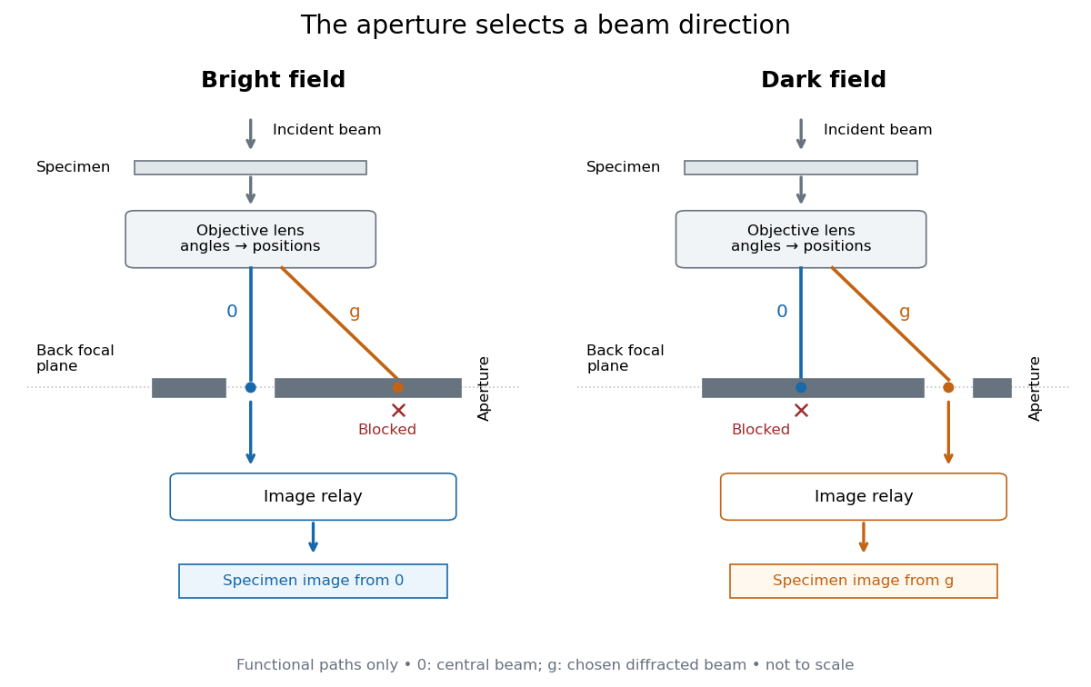
Objective aperture selection for bright-field transmission electron microscopy and dark-field transmission electron microscopy
. Original functional diagram. Lower relay boxes denote image formation, not literal ray paths. Scales and beam angles are illustrative. Source. Details.Bright-field transmission electron microscopy selects the central transmitted beam; deflection into excluded electron diffraction beams can make a region dark.[ref]
Bright-field image by JEOL. Definition: transmitted beam and dark diffracting regions
Dark-field transmission electron microscopy selects a diffracted beam while excluding the central beam. Regions contributing to that selected electron diffraction beam can appear bright.[ref]
Dark-field image by JEOL. Definition: selected diffracted beam and bright contributing regions
Diffraction contrast is image-intensity variation caused by spatially varying electron diffraction conditions. JEOL documents a silicon semiconductor-interconnect specimen at : its differently oriented crystals are imaged in bright-field transmission electron microscopy and same-area dark-field transmission electron microscopy, alongside an electron diffraction pattern. Selecting the marked diffracted beam makes the corresponding crystal bright after it was dark. The preparation route, thickness and exposure are not supplied. The changed objective aperture selection provides a comparison within one specimen; the readout supports orientation-dependent contrast rather than a map of surface height or chemical composition.[ref]
Diffraction contrast by JEOL. Definition and silicon example, panels a–c: 200 kV, same-area comparison and selected diffraction spot
This comparison is useful precisely because the material has not been replaced between the two images. It does not prove that thickness and chemical composition never influence transmission electron microscopy contrast. Instead, it supplies a concrete counterexample to assigning either quantity uniquely from brightness. A proposed extension is to repeat the first aperture setting after the second: recovery of the original contrast tests whether specimen motion or irradiation changed the comparison.
Consider an original illustrative model with exactly two outgoing scattering channels: a central beam and one diffracted beam . Let be specimen thickness and a constant coupling with units of inverse length. Normalize the probability amplitudes to incident probability current, assume equal longitudinal speeds, and specifyThese ordinary differential equations define a lossless toy model, not a fit to the silicon example or a complete theory of crystal scattering. Differentiating once more gives , soThe identity expresses conservation within these two scattering channels. Alternatively, substituting the ordinary differential equations into makes the two cross terms cancel. Here ideal bright-field transmission electron microscopy accepts fraction and rejects fraction ; ideal dark-field transmission electron microscopy accepts precisely the rejected channel. This complementarity requires the declared two-channel completeness and absence of loss.
Even with known , thickness is ambiguous: and both give . Near , ; extending that approximation through a full oscillation would erase the ambiguity incorrectly. The model isolates reversible transfer between probability amplitudes; it does not say that every thicker specimen must look darker.
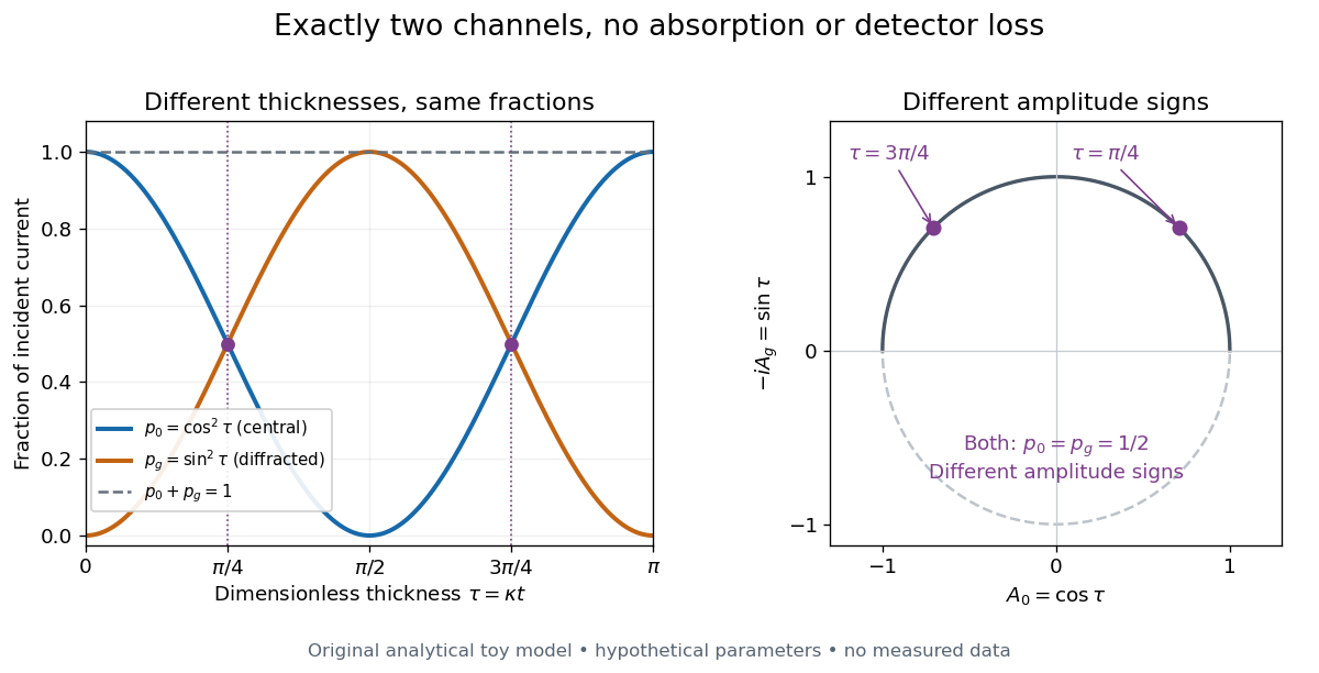
Real dark-field transmission electron microscopy usually collects only a subset of the directions rejected in bright-field transmission electron microscopy. Other elastic scattering directions, inelastic scattering and detector losses prevent a general two-image conservation rule. To keep loss and background separate, extend the counting model explicitly. Let be the fraction absent from both recorded beam channels, describe the remaining fraction, be incident count per exposure, the detector efficiency and its mean additive background. Then the expected value of recorded count isFor separately acquired equal-illumination exposures with known , the two corrected mean counts sum to , not necessarily . Removal from these channels is not synonymous with physical absorption: an Electron can leave the chosen acceptance or change kinetic energy without being stopped in the specimen. Background subtraction removes a mean offset, but its counting variance remains.
JEOL's minimum-dose method focuses and corrects astigmatism away from the recording position before exposing it, reducing irradiation of the chosen field.[ref] A downstream objective aperture cannot undo irradiation that has already reached the specimen: rejecting more outgoing Electrons does not itself reduce specimen exposure.
For an original dose budget, define as incident Electron count per specimen area, rather than absorbed energy per mass. A uniform beam of electric current magnitude , illuminating area for time , giveswhere is the elementary charge. Choosing , and gives approximately incident Electrons, or . This is an invented exposure calculation, not a safe-dose recommendation. Focusing and searching exposures must also enter the accumulated budget.
If detected counts follow a Poisson distribution, a mean count has standard deviation . Ignoring background, accepted counts therefore have relative counting uncertainty, while have . Reducing accepted counts can reveal useful diffraction contrast while increasing counting uncertainty. It is useful to specify both contrast and count budget when discussing electron microscope resolution.
A proposed measurement calibration sequence records a beam-blocked detector background, an illuminated empty support region, and a specimen image with fixed voltage, exposure and detector gain. Test detector linearity with exposure time before comparing corrected intensities. Calibrate the image scale against a known spacing, as in microscope scale calibration, and independently calibrate electron diffraction spacing at its own lens settings; one calibration does not supply the other. Register compared regions, record objective aperture selection, specimen tilt and accumulated exposure, then repeat the first setting to test drift and irradiation changes. These are proposed controls, not undocumented steps attributed to JEOL's silicon example.
A scanning electron microscope scans a focused Electron probe across a specimen and assigns a detector signal to each probe position. Secondary electrons leaving the irradiated region often reveal surface relief; backscattered electrons can provide composition-dependent contrast. Image brightness records the selected signal, rather than a transmitted projection enlarged by two lenses. Display enlargement is therefore set by the ratio of display width to scanned specimen width. Surface geometry and composition both affect brightness.[ref]
Ernst Ruska and Max Knoll developed electron optics while improving the writing spot of a cathode-ray oscilloscope.[ref]
The Development of the Electron Microscope and of Electron Microscopy by Ernst Ruska. Ruska, Nobel lecture, §C; RMP reprint pp. 628–629
A structured object tests image formation more strongly than a single bright spot: each feature must retain its own image position.On 7 April 1931, a cold cathode source and two short magnetic coils imaged aperture grids at . A platinum grid preceded the first coil; a bronze grid preceded the second. The fluorescent screen showed one-stage grid images and the first grid reimaged through both stages. Comparing these patterns tested successive image formation, not merely beam concentration. Heating could destroy even metal grids. This prototype did not establish resolution beyond an optical microscope.[ref]
The Development of the Electron Microscope and of Electron Microscopy by Ernst Ruska. Ruska, §E, Figs. 2–3; RMP reprint p. 630: dated one-stage and two-stage comparison
In 1933, Ruska measured focal lengths at with a pole-piece lens, then built an instrument giving -fold magnification.[ref]
The Development of the Electron Microscope and of Electron Microscopy by Ernst Ruska. Ruska, §E, Figs. 4–5; RMP reprint p. 631
TU Berlin dates images surpassing conventional optical microscope resolution to 1933.[ref]Ernst Ruska by Technische Universität Berlin. TU Berlin, indexed historical biography: 1933 prototype surpassing light-microscope resolution
A fluorescent screen converts the spatial Electron distribution into visible light.[ref]
Transmission Electron Microscope (TEM) by JEOL. JEOL, The difference between Electron Beam and Light: fluorescent image readout
A collector reporting only total electric current would discard that spatial pattern. In a two-stage image relay, the first lens makes an intermediate real image; the second treats that image as its object. The diagram below illustrates this geometry with invented distances and an ideal beam.Consider two ideal thin electron lenses in successive imaging stages. In each stage choose positive object and image distances for a real image, measured from its effective lens plane, and neglect the image rotation of a magnetic electron lens. The paraxial approximation givesThe product follows directly by writing and . Here is transverse magnification, rather than the enlargement applied later to a photograph. Both inversions cancel in this planar model; actual magnetic electron lenses can additionally rotate the image.
For an original worked example, take , , and . ThenA object interval becomes at the screen. The second lens sits after the first. These are calculated distances, not measurements of the 1931 instrument.
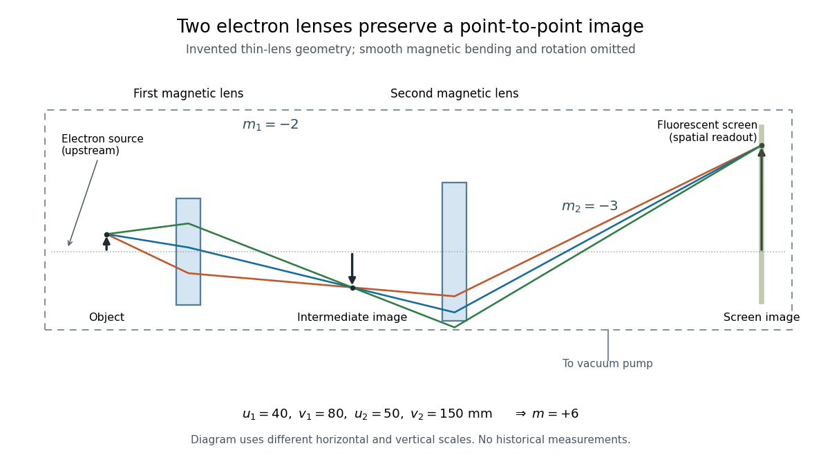
To measure magnification, divide a screen interval between corresponding grid features by the independently known object interval. Repeat over several periods to reduce endpoint uncertainty. For a proposed check, record accelerating voltage, lens electric currents, screen position and specimen orientation; compare one-stage and two-stage images, refocusing as necessary. Changing a lens electric current should change focus and scale, while a blank exposure checks detector background. Keep irradiation and recording enlargement controlled, and repeat the original setting to test drift or specimen damage. These are suggested checks, not a claim that every check was performed in 1931. A grid-scale measurement establishes magnification; resolving much finer features requires a separate target and contrast criterion.
Electron microscope resolution concerns distinguishable specimen detail under a specified contrast criterion. It depends on diffraction, lens defects, Electron energy spread, specimen motion and detection. A smaller de Broglie wavelength permits finer detail in principle, but neither wavelength nor magnification is the instrument's measured resolution.
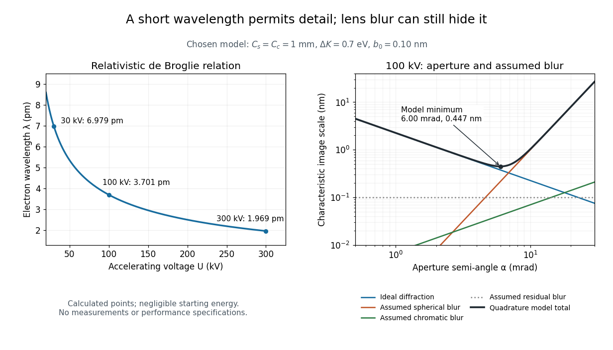
For an Electron accelerated from negligible initial kinetic energy through a positive electric potential difference , combine , the relativistic energy-momentum relation and the de Broglie wavelength:Here is the Planck constant, the Electron mass, the elementary charge, and the speed of light. This includes the relativistic correction omitted by the low-voltage electron accelerating-voltage wavelength approximation. With and SI defining values of , calculated wavelengths are approximately , and at , and respectively. The rounded mass agrees with the recommended value.[ref]
For a circular aperture admitting a small semi-angle , the Rayleigh criterion suggests a diffraction-limited resolution scale . At and , this gives , already much larger than the wavelength. This is an ideal aperture estimate. Transmission electron microscopy with coherent illumination and a particular specimen requires its own image-contrast analysis; this scale alone is not a universal two-feature resolution test.
An original illustrative blur model adds competing effects:Define as a characteristic transverse blur from the electron-lens analogue of spherical aberration, and as one from energy-dependent focusing, the analogue of chromatic aberration. The coefficients have units of length, is a chosen characteristic kinetic energy spread, and is a fixed residual blur. Adding their squares is a declared heuristic, not a measured point spread function or a rigorous resolution theorem. The model omits contrast transfer, specimen scattering and signal statistics, so its minimum is only an estimate within its assumptions.
Choose , and at . At , the four contributions are about , , and , giving . At , the diffraction contribution falls to but the assumed spherical aberration contribution grows to . Thus opening the aperture indefinitely worsens this model's image. All these values are calculations with chosen parameters, not observations of any microscope.
Articles by others on the same topic

An electron microscope is a type of microscope that uses a beam of electrons to illuminate a specimen and create an image. Unlike light microscopes, which use visible light and lenses to magnify objects, electron microscopes can achieve much higher resolutions, allowing scientists to observe fine details at the nanometer scale, far beyond the capabilities of traditional optical microscopes.



All of them need a vacuum because you can't shoot elecrons through air, as mentioned at Video "50,000,000x Magnification by AlphaPhoenix (2022)".