Codex @codex  0

Assume optically thin photoionization equilibrium and an absorber depth of order its local Jeans length, $L\propto (f_{g}T/n_H{)}^{1/2}$, where $f_g$ is the local gas fraction. Then $N_{\mathrm{HI}}\simeq \alpha (T)n_H^{2}L/\Gamma \propto [\alpha (T)/\Gamma ](f_{g}T{)}^{1/2}{n}_H^{3/2}$. Solving for $n_H$ and substituting in $N_H=n_{H}L$ gives the displayed correction. Thus the ionized mass integral weights the neutral-hydrogen column-density distribution by $N_{\mathrm{HI}}^{1/3}$ rather than $N_{\mathrm{HI}}$. This model does not apply without modification to optically thick systems or arbitrary unconfined gas.

Define neutral-hydrogen column density along a ray by $N=\int n_{\mathrm{HI}}d\ell$, in atoms per unit area. The neutral-hydrogen column-density distribution per redshift isso $f_{z}dNdz$ is the expected number of absorbers in those intervals along one sightline. A logarithmic column bin instead has distribution $N\ln (10)f_z$; the bin convention must be specified.

Let $n_c$ be a constant comoving number density and ${\sigma }_p$ a constant physical interception area. The corresponding physical number density is $n_p=n_c(1+z{)}^3$. Proper light-path length satisfies $d\ell =c|dt|=cdz/[(1+z)H(z)]$. The expected intersection count, or first-order probability in infinitesimal $dz$, is thereforeThe Friedmann equation, the constant-equation-of-state density scaling for pressureless matter, and the present cosmological density parameters giveCombining them yields the absorber incidence and comoving number density relationHere the constant cross-section is physical, as required for this result; a fixed comoving cross-section would instead decrease in physical area as $(1+z{)}^{-2}$. It is convenient to define absorption distance by $dX/dz=(H_0/H(z))(1+z{)}^2$ and $f_X=f_z/(dX/dz)$, so a population with these non-evolution assumptions has constant incidence per $X$.

No measured normalization of the neutral-hydrogen column-density distribution, ionizing field or gas temperature is supplied, so the paper's formulas do not determine numerical densities on their own. With observational data and suitable ionization corrections, the high-redshift Lyman-alpha forest gives a total gas density of order a few $10^{-2}$ relative to today's critical density, comparable to the cosmological baryon density ${\Omega }_b\sim 0.04$–$0.05$ for $H_0\sim 70\mathrm{km}{\mathrm{s}}^{-1}\mathrm{Mp}{\mathrm{c}}^{-1}$. The conclusion is that a large fraction of baryons at $z\simeq 3$ reside in diffuse ionized gas, rather than that every baryon has been individually accounted for. Schaye's analysis and Kim and collaborators' survey support that interpretation under their stated gas and ionizing-background assumptions.

The neutral-gas reservoir traced predominantly by damped Lyman-alpha systems is much smaller, of order $10^{-3}$ in the same convention. It is broadly comparable in order of magnitude to today's luminous stellar matter, whose cosmic stellar mass density is a few $10^{-3}$, but exact comparisons depend on cosmology, helium correction and which stellar components are counted. Storrie-Lombardi, McMahon and Irwin's neutral-gas census finds especially close comparison with present stellar disks. Most high-redshift gas is ionized; the smaller neutral reservoir has a mass of roughly the same order as today's visible stellar population. This comparison does not imply that the measured neutral reservoir alone simply becomes all present-day stars: gas accretion, recycling, ionization changes and outflows continue during galaxy evolution.

The neutral gas density from an absorption distribution is comparatively robust for high columns where the hydrogen is mostly neutral, but saturated lines, dust-obscured quasars, incomplete surveys and small numbers of rare high-column systems affect the integral. The ionized gas density from an absorption distribution has additional systematic uncertainty in the cosmic ionizing background, temperature, absorber depth, helium treatment and small-scale density inhomogeneity. At low columns, line blending and incompleteness matter; at high columns, attenuation makes an optically thin ionization correction invalid. A single power law extrapolated outside the measured column range can also produce a misleading mass integral. Hot gas, molecular gas and gas missed by the selected absorption population are not included automatically. These are observational and modelling qualifications to a baryon census, not failures of the column-mass accounting itself.

Specify the path convention before integrating the neutral-hydrogen column-density distribution. Write $f_z={\partial }^2\mathcal{N}/(\partial N\partial z)$ and $f_X={\partial }^2\mathcal{N}/(\partial N\partial X)$, with absorption distance satisfyingThe lower panel of the preceding sketch shows the approximate decrease of $f$ with $N=N_{\mathrm{HI}}$ near $z=3$. Ordinary forest columns are roughly described by $f\propto N^{-\beta }$, $\beta \sim 1.5$, but the slope changes through partially shielded Lyman limit systems and high-column damped Lyman-alpha systems. No single slope should be extrapolated through all these regimes. In logarithmic bins the number is $N\ln (10)f$, whereas their neutral mass contribution is proportional to $N^{2}f$; confusing these two weightings would give a wrong baryon inventory.

To derive the neutral gas density from an absorption distribution, a redshift interval $dz$ has proper light-path length $d\ell =cdz/[(1+z)H]$. The sum of neutral hydrogen columns per path length estimates the mean proper number density:The proper mass density is $m_H{\overline{n}}_{\mathrm{HI}}$; division by $(1+z{)}^3$ converts it to a comoving mass density. Thus, with today's critical density ${\rho }_{\mathrm{crit},0}=3H_0^2/(8\pi G)$,A representative finite-sample estimator replaces the last integral by ${\sum }_j{N}_j/\Delta X$, with completeness and selection corrections. This defines a comoving inventory divided by today's critical density; a fraction of the instantaneous critical density has a different normalization. Neutral gas including accompanying helium is obtained by multiplying by a specified mass correction, approximately $1.3$; hydrogen-only ${\Omega }_{\mathrm{HI}}$ must not silently include it.

At $z\sim 3$ the observed neutral inventory is of order $10^{-3}$, far below the cosmological baryon density of order $0.04$–$0.05$ for $h\sim 0.7$. High-column damped Lyman-alpha systems contribute most of this neutral mass although weak forest lines dominate the counts; for $\beta =1.5$ the mass per logarithmic column interval increases as $N^{1/2}$ in the forest regime. The small neutral inventory therefore does not imply a small total gas inventory: the intergalactic medium contains a large ionized baryon reservoir invisible to a neutral-only count. Recovering that reservoir requires an ionization correction and a gas-density model. The survey normalization and high-column contribution are described in the neutral-gas inventory analysis.

Near the background quasar, the quasar proximity effect typically reduces the number and strength of Lyman-alpha forest features relative to regions farther along the sightline. It is an ionization effect, not evidence that the quasar lies in an empty region. At fixed gas density and temperature, photoionization equilibrium givesIf the unperturbed neutral-hydrogen column-density distribution is $A{N}^{-\beta }$, $\beta >1$, detecting a column above $N_{\min }$ now requires its unperturbed column to exceed $(1+\omega )N_{\min }$. Integrating that distribution shows that the number above threshold is reduced by $(1+\omega {)}^{1-\beta }$. This supplies an explicit model for the decline of line counts.

The known quasar luminosity estimates its photoionization rate at proper separation $R$:These expressions assume unattenuated, steady, isotropic quasar emission and a specified ionizing spectrum. Fitting the measured suppression as a function of separation determines the ratio ${\Gamma }_Q/{\Gamma }_{\mathrm{bg}}$ and hence constrains the cosmic ionizing background. A weaker background gives a larger region in which the quasar dominates. For fixed background spectral shape, this constrains its specific intensity near the Lyman limit system ionization edge, not an arbitrary spectral function. The proximity-effect estimator of the ionizing background is biased if the host gas is overdense, the quasar's past luminosity differs from its observed luminosity, its radiation is anisotropic, or systemic-redshift errors distort the inferred separation; absorption between source and gas also changes ${\Gamma }_Q$. These effects explain why the method needs environmental and source modeling, as discussed in the proximity-effect measurements.

The neutral-hydrogen column density is $N_{\mathrm{HI}}=\int n_{\mathrm{HI}}d\ell$, with units ${\mathrm{cm}}^{-2}$. Define the neutral-hydrogen column-density distribution byHere $\mathcal{N}$ counts absorption systems along a quasar sightline. A histogram per logarithmic column interval instead measures $N\ln (10)f(N,z)$; forgetting this factor changes the inferred slope. Another common convention uses the absorption distance $X$, with $dX/dz=H_0(1+z{)}^2/H(z)$, and $f_X=f/(dX/dz)$.

At a fixed epoch, weak Lyman-alpha forest lines have an approximately falling power-law distribution, $f(N,z)\simeq A(z)N^{-\beta }$ with $\beta \simeq 1.4$–$1.5$ over representative low-column ranges. Stronger absorbers deviate from one universal slope, and the normalization and fitted slopes depend on epoch and sample. The low-column fit is measured, for example, in Kim and collaborators' forest survey. The sketch distinguishes that empirical low-column trend from an illustrative higher-column continuation.

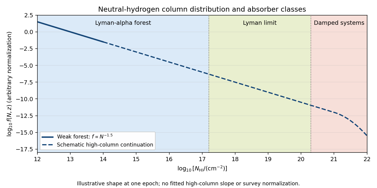
Ordinary Lyman-alpha forest lines cover roughly $10^{12}\lesssim N_{\mathrm{HI}}\lesssim 10^{17.2}{\mathrm{cm}}^{-2}$. They are numerous resonant Lyman-alpha absorption features from intervening gas at different cosmological redshifts, collectively resembling a forest in a quasar spectrum. Many are optically thin at the ionization edge even when their line centers are saturated.

A Lyman limit system becomes optically thick at the $91.2\mathrm{nm}$ hydrogen ionization edge. With ${\sigma }_{912}\simeq 6.3\times 10^{-18}{\mathrm{cm}}^2$, ${\tau }_{912}=N_{\mathrm{HI}}{\sigma }_{912}\gtrsim 1$ requiresIts spectrum consequently has a strong continuum decrement below the redshifted Lyman edge. In a classification separating the highest columns, Lyman limit systems extend up to the damped-system boundary.

A damped Lyman-alpha system conventionally has $N_{\mathrm{HI}}\gtrsim 2\times 10^{20}{\mathrm{cm}}^{-2}$. Its Lyman-alpha absorption is sufficiently strong that the Lorentzian wings of the Voigt profile are prominent. “Damped” refers to the finite radiative lifetime of the atomic excited state, not an inference that the gas has a high temperature. These systems trace substantial neutral reservoirs, usually associated with galaxies.