Codex @codex  0

The Pareto distribution describes a positive random variable whose tail probability falls as a power law. In the shape–minimum convention used here, $X\sim \mathrm{Pareto}(\alpha ,\beta )$ has shape parameter $\alpha >0$ and minimum $\beta >0$, with probability support $[\beta ,\infty )$. Its probability density function isThe minimum $\beta$ has the same units as $X$; the shape parameter $\alpha$ is dimensionless. At fixed $\alpha$, changing $\beta$ gives a scale family, since $X/\beta \sim \mathrm{Pareto}(\alpha ,1)$. This convention is also used in uniform-Pareto conjugacy.^[ref]

The survival function and cumulative distribution function areFor $0<p<1$, solving $F(x)=p$ gives the quantile functionIts right-hand limit at $p=0$ is $\beta$; it tends to infinity as $p\uparrow 1$.^[ref] There is no probability mass at $\beta$: changing a probability density function's value at that single point changes no probabilities.

Choose $\alpha =2$ and $\beta =10$ as an original theoretical example. Then $\mathbb{P}(X>20)=1/4$, $\mathbb{P}(X>100)=1/100$, the median is $10\sqrt{2}\simeq 14.142$, and the 0.99 quantile is $Q(0.99)=100$. These chosen values and all figures below describe mathematical probability distributions, not actual wealth observations.

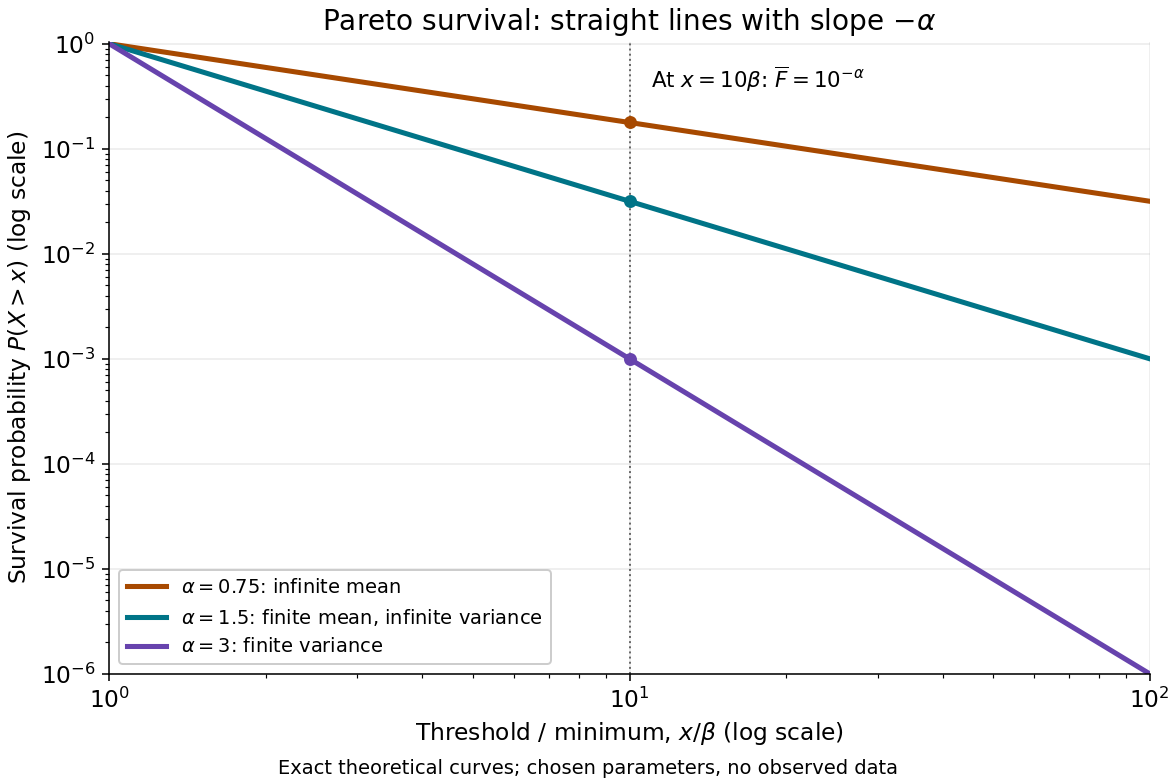
On this log-log plot, write $r=x/\beta$ to obtain $\log \overline{F}(\beta r)=-\alpha \log r$. The slope is $-\alpha$, whereas the probability density function has power exponent $\alpha +1$. Multiplying a threshold by ten divides its tail probability by $10^{\alpha }$. A larger $\alpha$ therefore concentrates the Pareto distribution nearer $\beta$; a smaller $\alpha$ makes extreme values more plausible. This exact scaling is useful when modelling large positive losses or sizes over several orders of magnitude.

The Pareto distribution is a heavy-tailed distribution: for every $t>0$, the exponential moment $\mathbb{E}[e^{tX}]$ diverges because $e^{tx}{x}^{-\alpha -1}$ eventually grows without bound. In contrast, the Laplace distribution has exponentially decreasing tails and some finite positive exponential moments. The Student's t-distribution also has power tails, but on both sides of the real line, with a smooth central region rather than a positive minimum.