Observable matrices in an energy basis ($A_{mn}=⟨m|A|n⟩$)

Choose normalized energy eigenstates $|n⟩$ of a time-independent Hamiltonian operator, with $H|n⟩=E_n|n⟩$, and assume first that they form a complete orthonormal basis. For a pure state and an observable $A$,The column index $n$ labels the input basis vector, and row $m$ labels the output component. Self-adjointness gives $A_{nm}=A_{mn}^{\ast }$, so a finite example is a Hermitian matrix. A matrix element can be negative or complex; by itself it is not generally a probability. The Born rule assigns measurement probabilities using the eigenstates of $A$, which need not be energy eigenstates. For an unbounded observable, these expressions require a suitable operator domain; a system with continuous spectrum also needs the corresponding spectral integrals.

In the Heisenberg picture, an observable without explicit time dependence hasHere $\hslash$ is the reduced Planck constant. An emitted photon on a transition $n\to m$ with $E_n>E_m$ has positive angular frequency $(E_n-E_m)/\hslash =|{\omega }_{mn}|$. The sign of the array's quantum phase follows its index convention; it is not a negative measured photon frequency. The frequencies involve differences of energy levels, rather than the absolute values $E_n/\hslash$. Adding a constant to $H$ leaves these frequencies unchanged.

Insert the complete orthonormal basis between two linear operators:The sum runs over intermediate states. The second identity follows by cancellation of $E_k$; it makes every term in the product acquire the same time factor $e^{i{\omega }_{mn}t}$. This is a useful reason for matrix multiplication: it composes the two indexed arrays consistently with the addition of transition frequencies. It does not multiply matching entries independently. Swapping $A$ and $B$ generally changes the intermediate-state sum and hence the result.

Consider an original ideal quantum system with positive scales $ϵ,d$ andInterpret $D$ as one component of an electric dipole moment, so its coupling to the corresponding electric field is the electric-dipole interaction $-\mathcal{E}(t)D$. The gaps are $2ϵ,3ϵ,5ϵ$, but $D_{02}=0$: this interaction has no direct first-order $2\leftrightarrow 0$ coupling. The nonzero squared matrix elements are $|D_{01}{|}^2=d^2$ and $|D_{12}{|}^2=4d^2$. These are coupling weights; actual spectral line intensities also depend on populations and radiation factors. In particular, there is no promise that an experiment populates the upper state of every allowed transition.

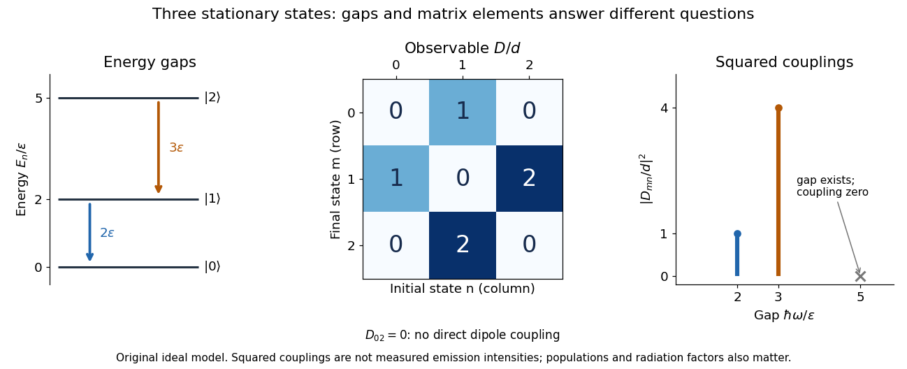
A measurement of $D$ itself has possible outcomes $0,\sqrt{5}d,-\sqrt{5}d$, sinceThese are eigenvalues of $D$, not the energy eigenvalues $0,2ϵ,5ϵ$. Moreover, $(D^2{)}_{02}=D_{01}{D}_{12}=2d^2$ although $D_{02}=0$: two factors connect through $|1⟩$. This algebraic statement does not turn $D_{02}$ into a nonzero direct coupling. Higher-order probability amplitudes for transitions require the appropriate dynamical calculation.