A quantum system is modeled by a complex Hilbert space; its quantum states describe preparations, while observables describe measurable quantities.
A quantum state describes a preparation through its predicted measurement in quantum mechanics probabilities. In the Hilbert space formulation, a pure state is a quantum state ray: a normalized vector representative satisfies , and representatives differing by a global phase describe the same quantum state. [ref]
Foundations I: States and Ensembles by John Preskill. Preskill, Foundations I: States and Ensembles, §2.1, printed pp. 1–3, equation (2.1) and the definition of a ray
Both pure states and mixed states are represented by a density operator on the chosen complex Hilbert space:Thus is Hermitian, positive semidefinite and of unit trace; in infinite dimension it must also be a trace-class operator. For a normalized pure state, is a rank-one orthogonal projection. A mixed state has no single such vector representative. Its density matrix is the matrix of in a chosen orthonormal basis. [ref]
Mathematical preliminaries. Watrous, The Theory of Quantum Information, §1.1.2, printed pp. 17–18, equations (1.94)–(1.97), Hermitian, positive semidefinite and density operators; finite-dimensional setting
For a discrete POVM with effects and , the Born rule readsThese constraints and Born rule probabilities describe arbitrary finite-dimensional preparations. [ref]Basic notions of quantum information. Watrous, The Theory of Quantum Information, §2.1.2, printed pp. 62–64, Definition 2.5 and pure states; §2.3, Definition 2.34, measurement probabilities
Randomly choosing normalized pure states with probabilities and forgetting the label givesThis quantum state ensemble averages probabilities; a quantum superposition adds probability amplitudes. Several ensembles can give the same density operator. Quantum entanglement can make a reduced density matrix mixed while the joint quantum state is pure. [ref]
Foundations I: States and Ensembles by John Preskill. Preskill, Foundations I: States and Ensembles, §2.3.1, printed pp. 14–18, equations (2.51)–(2.61), partial trace and ensemble interpretation
The preparation, the choice of basis, and the measurement are separate ingredients. A wavefunction is the position representation of a pure state; a general mixed state requires a density operator. For a closed quantum system, a unitary operator evolves it as , preserving its eigenvalues and purity of a density operator. [ref]
Foundations I: States and Ensembles by John Preskill. Preskill, Foundations I: States and Ensembles, §2.3.4, printed pp. 22–23, equation (2.79)
The Bloch sphere and Bloch ball give the qubit geometry; quantum state tomography connects repeated preparations to an estimated density matrix; projective measurement treats the conditional state after an outcome.A quantum state ray is the equivalence class of nonzero vectors in a complex Hilbert space under multiplication by a nonzero complex number. Its span is a one-dimensional linear subspace, but the zero vector is not a state representative. A unit vector fixes the norm and leaves a global phase free. [ref]
Foundations I: States and Ensembles by John Preskill. Preskill, Foundations I: States and Ensembles, §2.1, printed p. 2, ray equivalence and normalized representatives
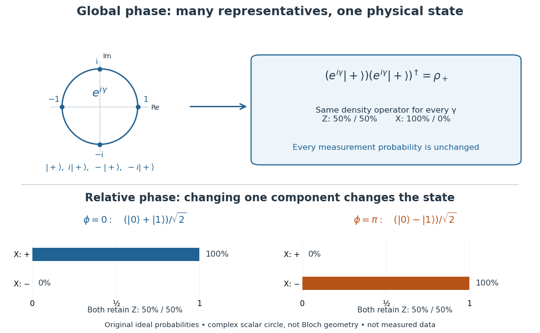
For a nonzero representative , the associated pure state density operator isReplacing by multiplies both numerator and denominator by , so the quotient is unchanged. In particular, for every POVM effect ,This proves that a global phase changes no measurement probability. Changing the relative quantum phase of two nonzero components can change the density operator, as the following comparison shows.
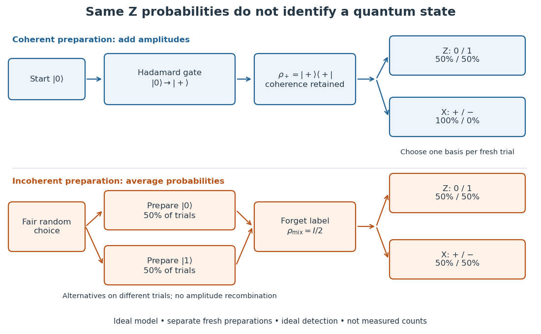
Choose the qubit computational basis , also called the basis, and the Hadamard basis , also called the basis. Compare a coherent preparation of with choosing or at random with equal probabilities and discarding that label:These are original ideal preparation models. Their -basis probabilities are both , because their quantum state populations agree. Their -basis probabilities are respectively and . Indeed , whereas . The missing off-diagonal quantum coherence therefore changes a prediction that the common populations cannot determine.

For a relative quantum phase , the coherent family instead hasThe last formula follows by adding or subtracting the two probability amplitudes before taking the squared modulus. At , the state is and the outcomes switch to , while the outcomes remain . In contrast, changes both components by the same global phase and retains the outcomes . In photon polarization, the identification , makes and the two orthogonal diagonal linear polarizations; these labels describe measurement bases, not spatial axes for photon spin.

Even perfect statistics in one basis cannot certify a preparation. The above data fit both density matrices. Conversely, distinct preparation histories can yield the same quantum state:The off-diagonal terms cancel in the right-hand ensemble. Every measurement on the qubit alone then has identical probabilities for those two histories. A retained classical label would allow conditioning on different members of the quantum state ensemble; it is extra information beyond the unlabelled density operator.
A 2018 photonic experiment makes the distinction between populations and quantum coherence controllable. A 400-nm laser pumped a crystal to generate paired photons, filtered near 800 nm. One photon triggered collection; the other entered the apparatus. A half-wave plate and polarizing beam splitter selected horizontal photon polarization; another half-wave plate prepared balanced quantum superpositions. Separated polarization paths and diffraction gratings let a spatial light modulator control their frequency-dependent quantum phases and spectral weights. Recombined paths passed through quartz plates whose adjustable thickness controlled polarization–frequency coupling. Quarter- and half-wave plates plus a polarizing beam splitter selected tomography bases; jointly registered photodetector events supplied the readout. Quantum state tomography inferred polarization density matrices at each thickness. The dephasing model preserves diagonal populations while changing off-diagonal quantum coherence. Here the unobserved photon frequency acts as the environment for the polarization qubit. Finite modulator resolution and imperfect spectral shaping limited agreement with the intended dynamics; this experiment does not establish exact preparation or the ideal probabilities above. [ref]
Experimental implementation of fully controlled dephasing dynamics and synthetic spectral densities by Zhao-Di Liu and others. Experimental implementation of fully controlled dephasing dynamics and synthetic spectral densities, Nature Communications 9, 3453 (2018), Results: Experimental setup, Fig. 1, equations (1)–(5); Using a photon to simulate qubit coupled to Ising chain, systematic-error discussion after Fig. 3
The -qubit Dicke state with excitations is the normalized equal superpositionwhere is the Hamming weight in the computational basis. The binomial coefficient counts the mutually orthogonal summands, proving normalization. Every permutation of the qubits leaves the vector unchanged. Splitting the sum according to the first bit and using givesTerms with zero coefficient are omitted at the endpoints. This recursion is useful for partial traces and for distributing a logical qubit among many symmetric physical qubits.
The -qubit W state is the Dicke state with one excitation:For three qubits it is . Its reduced density matrix on any one qubit is , from the Dicke state recursion. For both diagonal entries are nonzero, so that qubit is entangled with the rest: a pure product state would have a pure marginal. A symmetric-arm reduction of an exchange Hamiltonian supplies a dynamical preparation from one initial excitation.
For , and , the reduced density matrix of any one qubit isUse the Dicke state recursion. The rest-of-system vectors of different Hamming weights are orthogonal. For the diagonal terms this leaves the probabilities of the distinguished bit being zero and one. In the cross term, only the rest vector occurs in both states, with coefficients multiplying and multiplying . Thus , proving the matrix. A single Dicke state alone gives the diagonal matrix .
A flavor eigenstate is a state with a definite flavor label in the specified interaction or flavor-charge basis. For neutral kaons, and have definite opposite strangeness. Weak interactions mix them, so these flavor states are not the mass eigenstates. The precise flavor basis must be specified when discussing mixing.
A quantum superposition is a linear combination of quantum state vectors in a complex Hilbert space. In a specified orthonormal basis, a normalized pure state has the displayed expansion, where are probability amplitudes. A nonzero linear combination can always be normalized; an arbitrary sum of normalized vectors need not already have norm one. Having more than one nonzero component depends on the chosen basis: the Hadamard basis vector is a quantum superposition of the two computational-basis states, but is a single vector of the Hadamard basis. [ref]
https://ocw.mit.edu/courses/8-04-quantum-physics-i-spring-2016/7f930e013cef9cd7dec5aa88baa83f0a_MIT8_04S16_LecNotes1.pdf. Zwiebach, MIT 8.04, lecture 1, section 4, pp. 10–12
.The distinction from classical ignorance is quantitative. Consider the normalized qubit quantum stateIts density operator, written in the computational basis, isPreparing with probability and with probability , while discarding the preparation label, instead gives the mixed stateThe diagonal entries agree, so both preparations give the same computational-basis measurement probabilities. The off-diagonal entries of retain quantum coherence and the relative quantum phase. In the Hadamard basis, the Born rule givesThe density matrix representation retains this distinction between a pure state and a mixed state. [ref]
https://quantum.cloud.ibm.com/learning/en/courses/general-formulation-of-quantum-information/density-matrices/density-matrix-basics. Watrous, IBM Quantum Learning, Density matrix basics, Interpretation of density matrices and Connection to quantum state vectors
.For example, at , the quantum superposition yields the plus outcome with probability about , whereas the mixed state yields it with probability . At these particular probabilities agree, although the density matrices still differ: equality for one measurement does not establish equality of quantum states. The probability amplitude figure shows the comparison throughout a full cycle of relative quantum phase.
This is why a quantum superposition is useful: quantum gates act linearly on its probability amplitudes, and unitary operators preserve the full pure state information, including relative quantum phases. A Hadamard gate can turn otherwise hidden quantum coherence into different outcome probabilities. The beautiful feature is that the same basis weights can support different predictions when amplitudes recombine. The expansion specifies a preparation and its measurement predictions; it does not assign every unmeasured outcome a simultaneous classical value. See projective measurement for the separate question of the conditional state after a measurement.
A qudit is a quantum subsystem with distinguishable basis states and Hilbert space . A qubit is the special case . Tensor products of qudits give a natural setting for local Hamiltonians and finite-dimensional quantum circuits.
For an -level qudit and primitive root of unity , these unitary operators obey and . The inverse of is , with the order reversed. These operators implement the receiver corrections in qudit teleportation.
A qubit, or quantum bit, is a quantum system whose state space is a two-dimensional complex Hilbert space. Choose an orthonormal basis , called the computational basis. A pure state has a normalized representative , where are complex probability amplitudes and . General qubit states, including mixed states, require a density matrix. [ref].
The abstract qubit describes the chosen degree of freedom: for spin one-half, can label spin up and down along a specified axis; for photon polarization in a fixed propagation mode, they can label horizontal and vertical polarization, . These implementations share the same two-dimensional linear algebra, but their preparation and measurement in quantum mechanics use different apparatus. A qubit therefore need not be an entire two-level particle. [ref]
Foundations I: States and Ensembles by John Preskill. Preskill, Physics 229 notes, sections 2.2.1–2.2.2, spin and photon polarization examples
.The usefulness of a qubit lies in controlling quantum superpositions and their relative quantum phases, then converting them into outcome probabilities with quantum gates and an appropriate measurement. One ideal computational-basis measurement returns one label, zero or one. It does not reveal both probability amplitudes, their relative quantum phase, or all the bits of a larger register's expansion. Quantum state tomography instead estimates a qubit state using many repetitions of the preparation and suitable measurement settings. [ref].
An actual preparation and measurement example is Dederick and Beck's 2014 teaching-laboratory experiment. A 405-nm laser pumped two nonlinear crystals, producing signal and idler photons near 810 nm. In their non-entangled run the source produced ; a quarter-wave plate in the signal arm changed its photon polarization to in their convention. The plate supplies a relative quantum phase between polarization components. An idler detection selected the signal trials; signal detectors measured horizontal/vertical, diagonal, and circular polarization bases on separate runs. Before the polarization analyzer, a half-wave plate at degrees selected the diagonal basis, and a quarter-wave plate at degrees selected the circular basis. Coincidence counts gave the conditional positive-outcome frequency . The reconstructed density matrix for conditioning on detector had squared quantum fidelity with and purity of a density operator : close to the intended pure state, rather than an exact ideal preparation. [ref]
https://people.reed.edu/~beckm/papers/Dederick_ajp.pdf. Dederick and Beck, Exploring entanglement with the help of quantum state measurement, American Journal of Physics 82, 962–971 (2014), sections II D and III A–B
.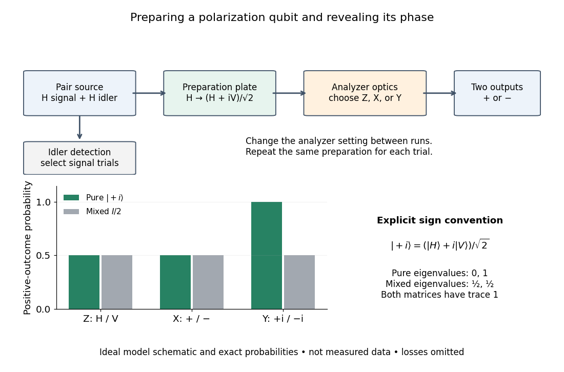

The model diagram explains why those settings matter. With and , the intended gives equal probabilities in both the horizontal/vertical computational basis and diagonal Hadamard basis, just as the mixed state does. In the circular basis , however, the ideal always gives the plus outcome, whereas still gives equal probabilities. These are deductions from the Born rule, not the paper's measured counts. Unequal detector efficiencies and finite samples must be accounted for when interpreting experimental frequencies; the ideal comparison assumes equally efficient detection.
A qubit state specifies measurement probabilities, rather than a pre-existing answer to every possible measurement. For a pure state, normalized vectors differing by a global phase represent the same physical state:Equivalently, the pure state is a ray: the one-dimensional complex linear subspace spanned by any nonzero representative. Dividing a nonzero vector by its norm fixes its length, but leaves the global phase free. The density operator is unchanged because . In contrast, multiplying only one nonzero component by changes a relative quantum phase and can change measurement probabilities. [ref].
After choosing a global phase, every pure state of a qubit can be writtenAt or , the parameter does not distinguish physical states: only one component survives. Elsewhere it is the relative quantum phase. The corresponding unit Bloch vector is on the existing Bloch sphere. Its angles describe a space of states; for a photon polarization qubit they are not the photon's position or direction of travel. [ref].
The Born rule in the computational basis gives and . These probabilities discard . In the Hadamard basis , adding or subtracting the probability amplitudes instead givesThis last equality follows by substituting the angular representative. In the basis , the same calculation givesThus both the real and imaginary parts of quantum coherence can be observed, using different measurement settings. For example, and both give , but the first gives and the second . A global phase could never cause this difference.
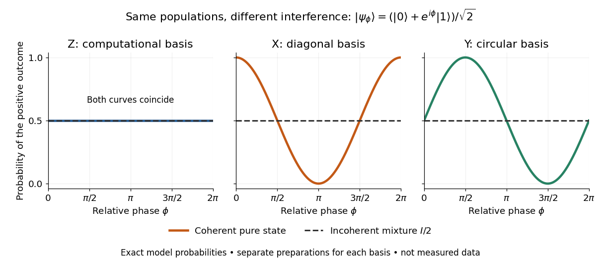
Identical computational-basis probabilities can hide different relative phases and coherence
. Exact model probabilities for , compared with the incoherent mixture . Each curve requires repeated preparations measured in the indicated basis; these are not experimental data. Details.
For a general qubit state, write its density matrix in the computational basis asThese are exactly the Hermitian, unit-trace, positive semidefinite constraints. Positivity means every eigenvalue is nonnegative, not that every matrix entry is nonnegative. The general definition is given in density matrix. [ref]
https://quantum.cloud.ibm.com/learning/en/courses/general-formulation-of-quantum-information/density-matrices/density-matrix-basics. Watrous, IBM Quantum Learning, Density matrix basics, Definition and Connection to quantum state vectors
.For this two-by-two matrix, the explicit constraint follows from its determinant, : with trace one, a nonnegative determinant and real eigenvalues rule out a negative eigenvalue. Its eigenvalues areThe pure states have and eigenvalues ; the mixed states have strict inequality and two positive eigenvalues. For a normalized representative, and . A statistical preparation , with and , averages probabilities, rather than adding probability amplitudes. Such a preparation is mixed if the positive-weight vectors do not all represent the same ray. A reduced density matrix of an entangled pair can also be mixed even when the pair has a pure state. [ref]
https://quantum.cloud.ibm.com/learning/en/courses/general-formulation-of-quantum-information/density-matrices/density-matrix-basics. Watrous, IBM Quantum Learning, Density matrix basics, Interpretation of density matrices
.For a concrete check, the pure state and the mixed state obtained by preparing with probability and with probability haveBoth have trace one and the same computational-basis measurement probabilities. Their eigenvalues are respectively and ; the respective values of their purity of a density operator are and . Their Hadamard basis plus probabilities are respectively and . By contrast, setting would give determinant and eigenvalue : normalized diagonal entries alone do not make a valid qubit state.
The same constraints become especially beautiful in the Bloch ball representation. With the Pauli matrices and the identity operator ,The eigenvalues are , so the Bloch sphere is precisely the pure state boundary, and is the maximally mixed centre. For each axis , the Born rule gives . This unifies a geometric picture, matrix positivity, and experimental frequencies in one description. For the equatorial family in the phase diagram, and ; replacing it by erases the transverse components and every fringe. See quantum state tomography for how independent ensembles measured along the three axes estimate these components. [ref].
A qutrit is a three-dimensional quantum system, with pure states satisfying . A qubit-qutrit state is a bipartite state on .
A quantum number is a discrete label, usually an observable's eigenvalue, used to distinguish quantum states.
Multiplying a quantum state by one global complex phase does not change any measurement probability; relative phases between components can affect interference.
The global phase is common to the whole state; relative phases control interference between state components.
A geometric phase is a quantum phase associated with the geometry of a path of state rays, after separating the dynamical phase. The Berry phase is its cyclic case governed by the adiabatic theorem; more general cyclic evolution can also have a geometric phase.
For an energy eigenstate with instantaneous energy eigenvalue , the dynamical phase isIt comes from the Schrödinger equation and depends on the time spent evolving. In an ideal cycle under the adiabatic theorem, a periodic choice of instantaneous energy eigenstate gives , with Berry phase .
A global phase multiplies an entire quantum state by one complex number of modulus one. It does not change any measurement probability, unlike a relative phase between components.
A physical unitary gate used without coherent control gives the same quantum channel for and :Interleaving any preparations, known operations and measurements preserves this equality. Equivalently, each fixed measurement branch with uses gains only the overall factor , which cancels in its probability. Thus unrestricted repeated uncontrolled uses do not determine the common phase of the eigenvalues. A supplied controlled unitary gate is a different resource: changes by a relative control phase when is replaced by . Such controlled access permits quantum phase estimation to measure that phase relative to the identity branch.
A quantum observable is represented by a self-adjoint operator; its possible measured values are spectral values of that operator.
For a normalized state with finite second moment of a quantum observable , its uncertainty is the standard deviation of the measurement outcome: . This equals . The Robertson uncertainty principle bounds products of uncertainties using the expectation of the commutator.
The expectation value of a quantum observable is the expected value of its measurement outcome random variable in a specified quantum state. It predicts the mean of outcomes from many identical quantum state preparations. It need not equal any one possible outcome: for a spin one-half particle, equal probabilities of and give mean zero even though zero is never an outcome of that spin component. Here is the reduced Planck constant.
Let be a Hermitian operator on a finite-dimensional Hilbert space, and let be a normalized pure state, . The spectral theorem writesThe are distinct real eigenvalues, are orthogonal projections onto their eigenspaces, and is the identity operator. For an ideal projective measurement of , the Born rule and the expectation value giveThus the expectation value is a probability-weighted average of eigenvalues, including all vectors in a degenerate eigenspace in its . In an orthonormal eigenbasis, , this is , where repeated are allowed. The weighted average lies between the smallest and largest eigenvalues; it can lie in a gap between them. The statistical meaning and operator expression are connected in this way in the authored treatment of average energies.[ref]
Chapter 20: Operators. The Feynman Lectures on Physics, Volume III, Chapter 20: Operators, §20–2, equations (20.11)–(20.20): outcome frequencies, weighted mean, and operator expectation
If a nonzero vector has not been normalized, use ; the denominator is essential. A global phase cancels between the bra and ket, so and have the same expectation value and outcome probabilities.
The outcome variance measures the spread about this mean, whereas the quantum uncertainty is its standard deviation:For a pure state, zero variance means that lies entirely in one eigenspace. That eigenspace need not be one-dimensional. Knowing only a mean generally does not determine the entire outcome probability distribution.
For a mixed state, the same formulas use its density matrix , a positive operator with trace one:A pure state is the special case . For a quantum state ensemble , the expectation value is . This linearity is useful when preparations vary between trials; different quantum state ensembles can have the same density matrix.
These formulas require no operator-domain qualifications in finite dimension. For an unbounded self-adjoint operator, the spectral theorem instead gives a spectral probability measure; a finite mean requires an integrable absolute first moment, and finite variance requires a finite second moment. Writing as an operator inner product additionally requires in the operator domain of . The quadratic form of a positive quantum Hamiltonian explains the useful wider form-domain version.
For spin one-half, choose the normalized spin eigenstates with . The spin one-half along an axis pure state in the plane isIts norm is one because the two eigenstates are orthogonal and . Applying the Born rule to a projective measurement givesConsequently the expectation value, second moment, and variance areAt , the outcome probabilities are and , the mean is , and the variance is . Every individual outcome remains . At , the mean is zero and the variance is maximal, . At either pole, one outcome has probability one and the variance vanishes.
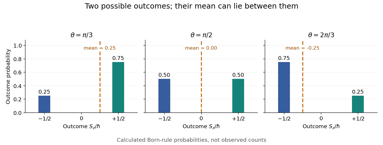
Spin expectation value between the two possible outcomes
. Original calculated Born rule distributions at three preparation angles. Bar heights are outcome probabilities; the dashed orange line marks the expectation value, whose horizontal position is usually not an allowed outcome. Spin values are expressed in units of the reduced Planck constant. No bars represent experimental observations. Source. Details.
The diagonal mixed state has the same probabilities, expectation value, and variance as . It is nevertheless a different quantum state for : the displayed pure state has , while has . A single component's mean does not reveal all relative quantum phases or establish purity of a density operator.
Prepare a fresh copy of the same quantum state for each trial and measure the same observable. If preparations and readouts are independent, the outcomes are independent and identically distributed random variables with the Born rule probability distribution. Their sample mean is an unbiased estimator of the expectation value:The law of large numbers explains convergence of the sample mean, while the standard error describes its finite-sample spread. It takes four times as many independent trials to halve that standard error. This reduces estimation error; it does not reduce the quantum uncertainty of a single prepared copy.
For the spin expectation value, let and be the two outcome counts, with . ThenThe binomial distribution gives the exact sampling model. For , the standard error is : approximately for and for . A run can fluctuate away from the predicted mean even as its typical spread decreases.
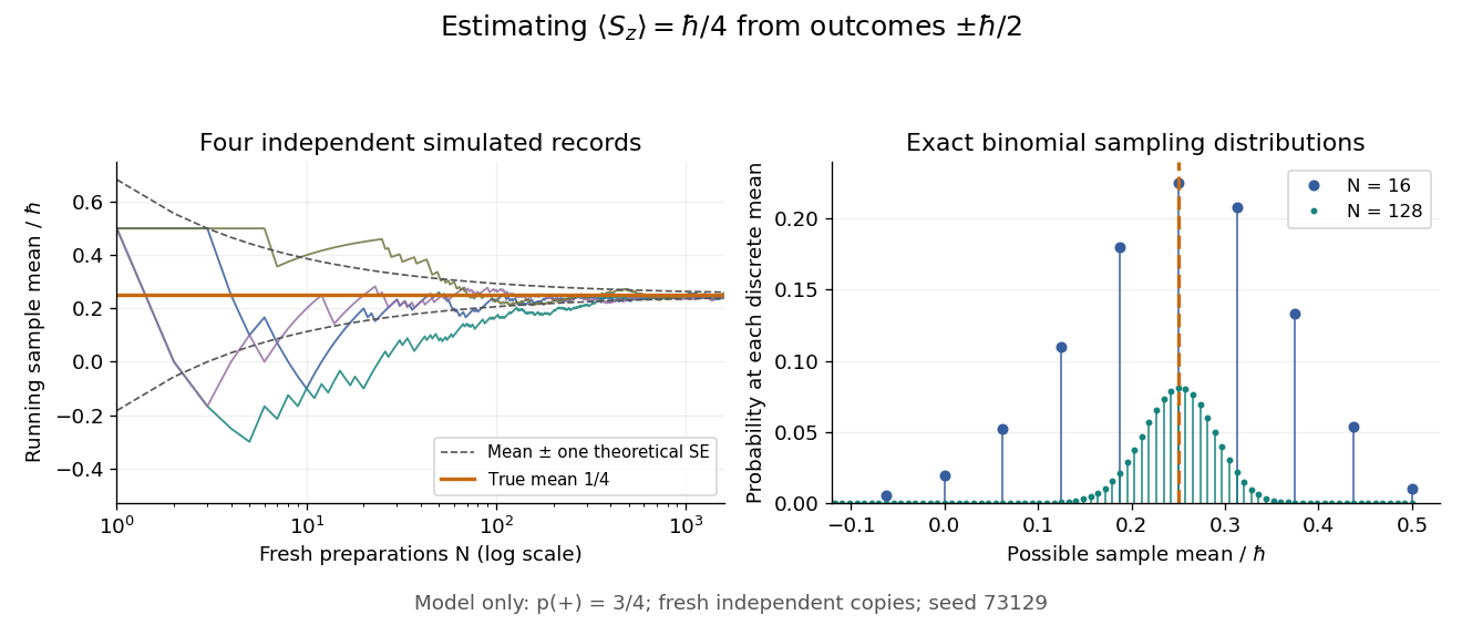

Repeatedly measuring one surviving system is a different protocol. Under the ideal Lüders rule, outcome leaves when . With no intervening change of observable or dynamics moving the state out of that eigenspace, the next projective measurement returns with certainty. Such a record is correlated and does not sample the original Born rule distribution independently. The quantum nondemolition measurement discussion describes this repeatability; fresh quantum state preparations supply the ensemble needed for the estimator above.
A concrete idealized implementation uses a Stern-Gerlach experiment twice: a preparation filter along passes only its plus spin channel, and a analyzer resolves both output channels for many fresh atoms. This prepares the spin one-half along an axis state . The authored apparatus description uses slit collimation, a nonuniform magnetic field with a pointed pole, and counters at the separated outputs.[ref]
Chapter 5: Spin One. The Feynman Lectures on Physics, Volume III, Chapter 5: Spin One, §5–1, figure 5–1 and the paragraph proposing output counters; §5–4, slit diffraction and internal-state limitations
The two-channel spin one-half preparation and analyzer are described separately; the source's recombining “improved” apparatus is explicitly idealized, so the setup here is a proposed estimation model, not a report of observed counts.[ref]Count every accepted analyzer event in its calibrated or channel and compute from the count difference. The magnetic field gradient separates trajectories through their magnetic moments; calibrated channel labels convert positions into spin eigenvalues. The readout is a population imbalance, not an intermediate trajectory carrying spin . Beam position also depends on flight time and field geometry, so averaging raw positions alone does not establish a calibrated spin expectation value.
As controls, feed known and preparations to check the channel assignment and leakage, hold the analyzer axis fixed, and repeat short blocks to check preparation drift. Measure background counts and relative channel efficiencies. With efficiencies and and negligible background, the detected plus fraction isUnequal efficiencies bias the naive sample mean, even for arbitrarily many counts. For example, , , and give detected fraction and naive mean , rather than . Background, overlapping beams, detector saturation, angle misalignment, unwanted internal states, and preparation correlations require a better measurement in quantum mechanics model. Increasing only reduces the independent sampling contribution; it cannot remove these systematic errors. The selected preparation beam is the population being estimated, so losses in preparing it must be distinguished from losses in reading its two outcomes.
The Hamiltonian operator represents the total energy and generates unitary time evolution through the Schrödinger equation.
For a positive self-adjoint Hamiltonian operator, finite energy means that a normalized state lies in , its form domain, and has expectation value . This domain can be larger than . With a complete orthonormal basis of energy eigenstates, and give by applying and taking its squared norm. Membership in instead requires . For a Dirichlet free-particle Hamiltonian operator on an interval, the energy form is on functions with square-integrable weak derivative and zero endpoint values.
The Morse potential models an anharmonic molecular bond with dissociation energy , equilibrium separation , and inverse length . Unlike a quantum harmonic oscillator, it has finitely many bound levels and a dissociation continuum.
The quantum Hamiltonian with kinetic energy and Morse potential has bound energies of the displayed form, where , and . Adjacent energy differences are , distinct and positive over the physical bound-level range. A finite truncation with nonzero adjacent dipole couplings therefore satisfies connected nondegenerate transition chain generates special unitary control. Controllability of such a truncation does not by itself prove controllability on the full space including dissociation states.
For with real and positive , the factorization gives potential and a nonnegative energy form. Its zero mode is proportional to . Taking and optimizing positivity over gives the Heisenberg uncertainty principle for states with finite second moments.
For real polynomial , , the zero mode of is normalizable on exactly when is odd and . Its squared modulus has leading exponential . Odd gives the same tail sign at both ends; positivity of makes both tails decay. This kernel is one-dimensional because is a first-order differential equation. On the operator domain where integration by parts is valid, the energy form is .
A unitary operator is a symmetry of a time-independent Hamiltonian whenequivalently . A differentiable one-parameter symmetry has a self-adjoint generator satisfying , so is conserved.
A Hamiltonian operator has perfect transfer between basis states at time if for a known global phase . In an excitation-conserving qubit network whose vacuum is fixed, the initial product state with at site and zeros elsewhere evolves to . A local phase gate at removing restores the unknown qubit there. This explains why transfer of the single-excitation basis state suffices for qubit transfer when the vacuum phase is also accounted for.
In the Schrödinger picture, states evolve with the Hamiltonian operator while observables without explicit time dependence are fixed. For time-independent , the corresponding Heisenberg picture operator is .
The time-evolution operator maps an initial quantum state to its state at a later time. For a time-independent Hamiltonian operator , it is the unitary operator .
A quantum-mechanical propagator is the position-space kernel of the time-evolution operator. It is the amplitude to evolve between the specified endpoint configurations.
In units , a particle of mass with potential has classical path . Its action and exact quantum-mechanical propagator areThe fluctuation operator is the free one because the potential is linear. This is a special case of classical-path factorization of a quadratic path integral.
For unit mass and , this prepoint kernel tends to the identity and generates the Time-dependent Schrödinger equation. The square-root branch follows the damped Fresnel integral. Its normalized moments are , , and at orders zero, one and two; these fix both the normalization and the kinetic sign.
Expand a smooth wavefunction and potential in the normalized short-time Schrödinger kernel. Its odd moment vanishes and its second moment is , so one step changes the wavefunction by . Division by the time step gives the Time-dependent Schrödinger equation.
A semiclassical propagator sums over classical paths joining its endpoints, weighted by their quadratic fluctuation determinants and phase indices. It is exact for quadratic actions.
Expanding a configuration-space path integral about a classical trajectory with fixed endpoints gives , where obeys homogeneous Dirichlet boundary conditions. The Gaussian functional integral contributes with the phase prescribed by continuation of the quantum-mechanical propagator. Relative to the free operator , the prefactor is . In a general potential the operator, and thus the prefactor, depends on the endpoints through . For a quadratic potential is constant and all higher fluctuation terms vanish, so the approximation is exact away from singular focusing times. At a zero mode the simple determinant formula requires a limiting prescription or a different treatment of the zero mode.
The Van Vleck determinant is the determinant of mixed endpoint derivatives of a classical action. It measures how nearby classical trajectories focus and supplies the fluctuation prefactor of the semiclassical propagator.
In the Heisenberg picture, states are fixed and an observable evolves asFor a time-independent Schrödinger-picture observable,
For an operator in the Heisenberg picture, differentiating the evolution operators gives in units . With no explicit operator time dependence, the second term vanishes. Applying this commutator identity to the canonical momentum and real scalar field gives their operator field equations.
For , the interaction picture moves the free evolution into operators and leaves states to evolve with . Its evolution operator is the time-ordered Dyson series.
A time-reversal operator intertwines forward and backward evolution:It must be antiunitary in ordinary quantum mechanics. Its conjugate linearity sends to , allowing it to commute with a time-reversal-invariant Hamiltonian rather than reversing the sign of its energy.
A quantum time-reversal operator is an antiunitary operator reversing spatial momentum and angular momentum. For a time-reversal-invariant Hamiltonian operator, its conjugation of makes it intertwine forward and backward unitary time evolution without reversing the energy spectrum. A scalar momentum eigenstate may transform as . With unit-modulus phases and a complete normalized basis, expansion of arbitrary states proves antiunitarity.
If a unitary satisfied , differentiation at zero would giveIt would map every energy to . A Hamiltonian unbounded above would consequently be unbounded below and have no stable ground state.
For antiunitary , conjugate linearity gives . Differentiatingtherefore yields . Time reversal maps an energy eigenspace to itself and creates no negative-energy instability.
A Coulomb bound state is a physical normalizable eigenfunction for an attractive potential , . For the usual regular boundary condition at the origin its energies are the displayed values, . The spherically symmetric states have orbital angular momentum zero; series-termination quantization of the Coulomb radial equation constructs them as a polynomial times a decaying exponential. Square integrability on the punctured radial interval alone does not replace the physical condition at the origin.
For a spherically symmetric bound state, write . The radial Coulomb equation gives the displayed recurrence. Choosing terminates it after degree , producing a nonzero continuous polynomial times an exponentially decaying function. Its three-dimensional norm is finite and can be normalized. The energy is . Continuity at the origin is compatible with the Coulomb cusp; no differentiability as a Cartesian radial function at the origin is asserted.
Articles by others on the same topic
There are currently no matching articles.