Past exam of the advanced fluid dynamics course of the University of Oxford / 2023 / 1

Take the inviscid limit of the Navier-Stokes equation, neglect gravity, and use ideal magnetohydrodynamics. The governing equations areThe continuity equation also gives $D_t\rho =0$. Write the first-order magnetic perturbation as $\mathbf{b}={\mathbf{B}}^{\prime }$ and linearize about the uniform stationary background:For a nonzero-wavenumber plane wave proportional to $e^{i(kz-\omega t)}$, the two divergence constraints imply $v_z=b_z=0$. The longitudinal momentum equation then gives $P^{\prime }=0$ for that mode, and ${\partial }_t{\rho }^{\prime }=0$ gives ${\rho }^{\prime }=0$ for nonzero $\omega$. Thus the propagating Alfvén wave is transverse. Its two independent transverse directions have the same dispersion relation.

The Linear Alfvén wave equations reduce toEliminating either amplitude givesFor $B_0>0$, the branch traveling along $+z$ has $\omega =k{v}_A$ and $\mathbf{b}=-\sqrt{{\mu }_0{\rho }_0}\mathbf{v}$. The opposite branch reverses that amplitude sign. Finite viscosity would additionally damp the motion; it is neglected in obtaining the real ideal dispersion relation.

Subtract the constant equilibrium magnetic energy density. Since ${\mathbf{B}}_0\cdot \mathbf{b}=0$, the perturbation densities areThe traveling-wave amplitude relation from part a givesThis is pointwise Alfvén wave energy transport for one traveling wave, not a claim that every superposition or standing wave has pointwise equipartition.

For the real fields written as $\mathbf{v}=\mathrm{Re}(\hat{\mathbf{v}}{e}^{i(kz-\omega t)})$ and similarly for $\mathbf{b}$, the period averages areThe factors one half distinguish a sinusoid's peak amplitude from its mean squared value; the same complex-vector convention also covers circular polarization of waves.

In ideal magnetohydrodynamics, the first-order electric field is ${\mathbf{E}}_1=-\mathbf{v}\times B_0{\mathbf{e}}_z$. Retaining its product with both the background and first-order magnetic field gives the Poynting vectorThe first term is transverse and oscillatory, with zero period average. The second is quadratic and transports wave energy. A potential quadratic ideal electric-field term $-\mathbf{v}\times \mathbf{b}$ vanishes here because the real traveling-wave fields are parallel or antiparallel.

For the $+z$ branch, $\mathbf{b}=-\sqrt{{\mu }_0{\rho }_0}\mathbf{v}$, soFor the opposite branch, its sign reverses. The averaged Poynting flux is the total wave energy density, including equal kinetic and magnetic shares, multiplied by the group velocity. This agrees with Alfvén wave energy transport. Although the flux in this expression is electromagnetic, it supplies the transport of both components of the coupled fluid-field wave.

In this question, the coefficient multiplying ${\nabla }^2\mathbf{B}$ is the magnetic diffusivity. Denote it ${\eta }_m$; it is the paper's $\eta$, with dimensions of length squared per time. If ${\eta }_{\mathrm{Ohm}}$ denotes electrical resistivity, then ${\eta }_m={\eta }_{\mathrm{Ohm}}/{\mu }_0$. The two conventions must not be interchanged.

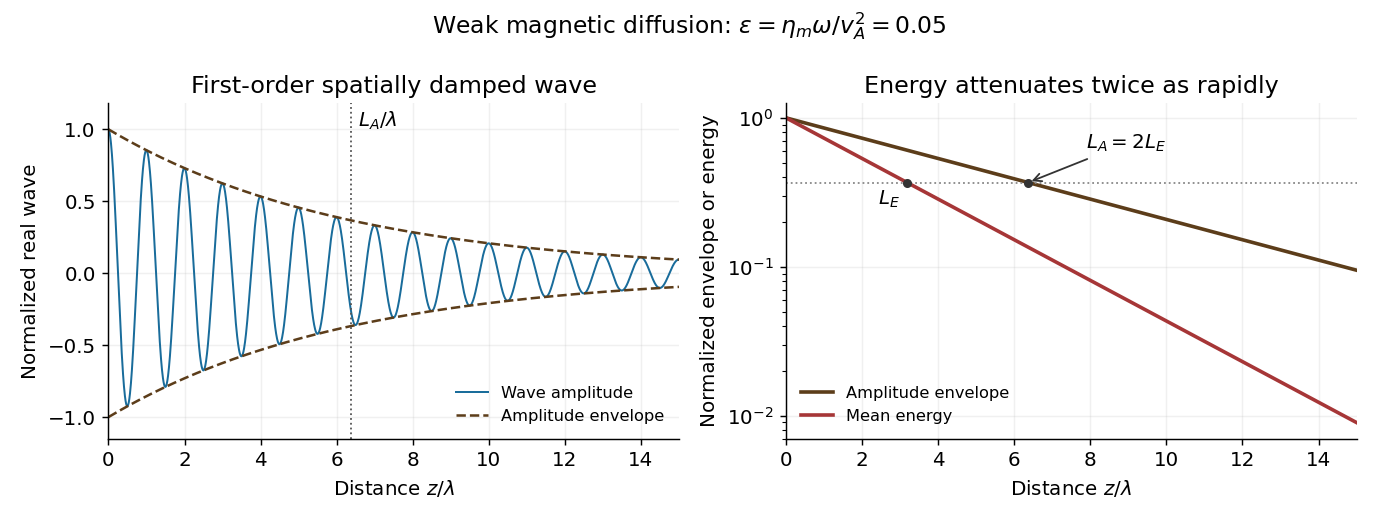
For an imposed real positive $\omega$, retain the momentum equation and useElimination gives the exact Resistive damping of an Alfvén wave relationHere $k$ is complex because the driving frequency is real. Introduce the dimensionless diffusion parameter $ϵ={\eta }_m\omega /v_A^2\ll 1$. For propagation and attenuation along $+z$, choose the square-root branch with $\mathrm{Re}k,\mathrm{Im}k>0$. The spatial damping of a driven Alfvén wave isWith the convention $e^{i(kz-\omega t)}$, the amplitude decays as $e^{-\mathrm{Im}kz}$. Define its e-folding length $L_A=1/\mathrm{Im}k$ and the wavelength $\lambda =2\pi /\mathrm{Re}k$. ThenIf damping length instead refers to wave energy, the squared amplitude decays twice as fast: $L_E=L_A/2$ and $L_E/\lambda \sim 1/(2\pi ϵ)$. Stating the convention avoids a factor-of-two ambiguity. The temporal damping rate ${\eta }_m{k}^2/2$ at fixed real $k$ is a different specification from this imposed-frequency problem.