Source PDF: mmathphys.physics.ox.ac.uk/sites/g/files/vzsiac2991/files/mmathphys/documents/media/a15271h1.pdf
Solutions to both questions and all nine parts. The two-sphere calculation uses the leading free-draining approximation, with negligible connector drag; the limitations of that approximation are made explicit.
To first order in fluid velocity divided by the speed of light, the Lorentz transformation of electromagnetic fields gives . Applying Ohm's law in the local fluid frame gives . Neglecting the displacement current in Ampère's law, . Substitution in Faraday's law givesHere is the magnetic diffusivity; the paper's is electrical resistivity, rather than magnetic diffusivity. Expanding the curl with the solenoidal magnetic-field constraint gives the resistive induction equation in its compressible form:The left side is the material derivative of the magnetic field. The three right-hand terms respectively describe field-line stretching and reorientation, amplification or dilution by compression or expansion, and magnetic diffusion. In particular, compression has and amplifies a field component perpendicular to the compression.
The assumptions are nonrelativistic bulk motion, the low-frequency approximation permitting omission of the displacement current, a conducting-fluid continuum, isotropic local Ohm's law with spatially constant scalar electrical resistivity, constant magnetic permeability , and . Hall, electron-pressure and other non-Ohmic corrections to the generalized Ohm's law are excluded. Incompressible flow is not required: imposing it would remove the compression term.
Let be the total magnetic energy. Multiply the curl form of the resistive induction equation by and integrate over the fixed volume. The identityfollows from the divergence theorem. The stated zero boundary fields remove its surface term. Applying it to the motional and resistive contributions yields the magnetic energy balance in resistive magnetohydrodynamics:The first term is the negative of the mechanical power delivered to the fluid by the Lorentz force density. It transfers energy between fluid motion and the magnetic field, with either sign. The second is the nonpositive magnetic contribution to Joule heating. A nonzero positive electrical resistivity therefore dissipates magnetic energy at rate ; it does not force the total magnetic energy to decrease when fluid motion supplies a larger positive power.
Choose a magnetic vector potential with . The resistive induction equation permits the evolution equationA gauge transformation changes by a surface integral of the normal magnetic field, which is zero here. Thus the integrated magnetic helicity has gauge invariance under the stated boundary conditions.
Differentiate both factors in . Use the stated vanishing-boundary assumption to remove the helicity surface flux; this can be implemented in the usual closed-boundary gauge , or by extending the localized field and integrating over all space with sufficient decay. The curl integration by parts identity then givesThe motional term is zero pointwise because . The scalar-potential term integrates to zero by and the boundary condition. The resistive magnetic-helicity balance is thereforeUnlike the resistive magnetic energy contribution, this signed integral need not have a fixed sign.
A magnetic field varying over a length has of order . Consequently, the resistive magnetic energy loss contains two inverse powers of , while the resistive magnetic-helicity balance contains only one. Small-scale gradients can therefore dissipate substantial magnetic energy while retaining an approximately conserved large-scale magnetic helicity.
A dimensionally consistent version is the selective decay bound for magnetic helicity. With , the Cauchy-Schwarz inequality givesFor bounded and bounded, possibly nonvanishing as , the resistive change in magnetic helicity tends to zero, even though resistive magnetic energy loss may remain finite. Magnetic energy is preferentially dissipated, while magnetic helicity is approximately conserved in this bounded-energy, bounded-dissipation limit.
This is not a comparison of quantities with different physical units or a universal ordering of fractional decay rates. For a single Beltrami field satisfying , both integrated quantities have fractional decay rate without fluid motion. The boundedness assumptions and distribution of magnetic helicity across spatial scales matter.
The stress tensor of the incompressible Newtonian fluid is , where is the rate-of-strain tensor. The homogeneous Stokes equations give . Apply the divergence theorem to the fluid between the body and a surrounding sphere . If points from the body into the fluid, the fluid-domain normal on the inner boundary is . HenceThis is the force flux at infinity in Stokes flow. A nonzero resultant force must be supported by a stress of order on a surface of area of order . More precisely, the leading exterior solution is a Stokeslet with force on the fluid :Thus , and . These are leading generic orders for a translating body with nonzero drag; the integral alone does not determine every angular component, and force-free disturbances may decay faster.
For two Stokes flows in the same fluid domain with the same dynamic viscosity, symmetry of the Newtonian fluid stress tensor and incompressibility give the local reciprocal identityIn index notation, its remaining cross-gradient terms are both . On the remote sphere the integrated reciprocal flux tends to zero: the velocity is , the stress tensor is and the area is . On the body, the no-slip boundary condition makes the two velocities the constants . The Lorentz reciprocal theorem therefore givesBy the Linearity of Stokes flow, the sum of the two velocity-pressure fields satisfies the boundary conditions for body velocity . Uniqueness of the exterior Stokes flow identifies it with the third solution. Since the stress tensor and its surface integral are linear too, ; scalar multiplication follows in the same way. Thus for a fixed-orientation hydrodynamic resistance matrix . Substituting arbitrary in the reciprocal identity yieldsThe minus sign is natural because viscous dissipation gives for nonzero rigid translation in an otherwise stationary fluid; is a positive-definite matrix.
Use the free-draining approximation: neglect the hydrodynamic interaction between the widely separated spheres and neglect the connector's viscous drag. Stokes law gives for each sphere. Their resultant isThis is the leading two-sphere approximation, not an exact finite-separation hydrodynamic resistance matrix. Writing and , the first Stokeslet reflection gives, if the connector remains negligible,The negative correction expresses reduced drag from fluid entrainment by the other sphere. A very thin but arbitrarily long rod need not have negligible total drag: its typical transverse drag scales as for rod radius . Thus the simple boxed result uses the intended negligibly dragging connector limit as well as ; the two printed size inequalities alone do not specify a uniform limit in which rod drag vanishes.
Hold the two-sphere object fixed in a uniform stream . In the free-draining approximation, its drag forces are , with . The hydrodynamic torque about isTo make it zero for every incoming-stream direction, choose the hydrodynamic centre of a two-sphere dumbbell:It lies closer to the larger sphere, whose larger drag requires a shorter lever arm. Uniform translation does not spin an isolated sphere, so no additional isolated-sphere spin torque enters this leading approximation.
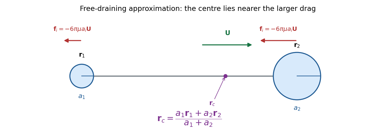
Finite-separation hydrodynamic interactions and connector drag can change the displayed location; the calculation has the same approximation as part c.
For rotation about the hydrodynamic centre of a two-sphere dumbbell, the sphere centres have velocities . Their resultant drag force in the free-draining approximation isEach sphere also experiences a spin drag torque, but its isolated rotation causes no net force. Those spin contributions therefore do not alter the cancellation.
This illustrates translation-rotation reciprocal coupling. About any fixed origin, write the fluid's rigid-body force and torque asThe transposed cross-blocks follow from the Lorentz reciprocal theorem. If pure translation causes zero torque about an origin for every , then , hence pure rotation about that origin causes zero force. This implication is general for linear Stokes flow; the existence and leading location of such an origin here use the two-sphere geometry and the approximation in part c.
Source PDF: mmathphys.physics.ox.ac.uk/sites/g/files/vzsiac2991/files/mmathphys/documents/media/advanced_fluid_dynamics_2024.pdf
Solutions to both questions and all nine parts. Part 2(d) contains a false identity in the source; its counterexample and the consistent free-energy balance are supplied.
Start in an inertial frame with the inviscid magnetohydrodynamic momentum equation,Here is mass density, is the isotropic fluid pressure, is inertial-frame velocity, is electric current density, is the magnetic field, and is gravitational potential per unit mass. In the low-frequency approximation to Ampère's law, . The vector calculus identityseparates the Lorentz force density into magnetic tension and a magnetic pressure gradient. Transform the material acceleration to a rigid frame rotating with constant angular velocity , using the stated frame transformation. The rotating-frame magnetohydrodynamic momentum equation isThe final terms are the Coriolis force and centrifugal force densities; is the velocity relative to the rotating frame, and uses that frame.
This requires a smooth conducting-fluid continuum with nonrelativistic motion, a constant magnetic permeability , the solenoidal magnetic-field constraint, a negligible displacement current and negligible net electric-charge force. Viscous forces and anisotropic fluid stresses are omitted. A time-dependent frame would add an Euler force. Incompressible flow is not needed for this force equation. Finite electrical resistivity does not change its displayed instantaneous magnetic force; the later frozen-field calculation additionally uses ideal magnetohydrodynamics. A differentially rotating fluid does not define a single rigid frame with spatially varying : choose a fixed local reference rate and retain the fluid's shear in .
In an inertial frame, a circular orbit at radius has radial acceleration . Neglecting fluid and magnetic forces givesIn a local rotating frame with , the fluid is instantaneously at rest at the reference radius . The radial centrifugal force then balances the inward gravitational force. Away from , the fluid's nonzero rotating-frame velocity must also be retained; the entire differentially rotating disk is not at rest in that one frame.
Take outward radial force as positive and keep the displaced element's angular rate fixed at . Its imbalance isUse the equilibrium relation from part b, , and a first-order Taylor expansion:The absolute values are needed for a magnitude. As printed, the proposed magnitude has a signed right side; it would be negative for outward displacement in a Keplerian disk. For decreasing , the signed imbalance above points outward and therefore amplifies that fixed-angular-rate displacement. This calculation fixes the angular rate, rather than the specific angular momentum; the latter is the conserved quantity for an uncoupled inviscid radial displacement and leads to the Rayleigh centrifugal stability criterion.
Linearized magnetic flux freezing gives the Eulerian magnetic field perturbationThe background is uniform, and incompressibility gives . For a horizontal displacement proportional to , and . Thus the first-order magnetic pressure perturbation vanishes, and the magnetic-tension response to an incompressible displacement isBending a field line produces a restoring force proportional to displacement, like a spring obeying Hooke's law. Per unit mass, its squared spring frequency is , where is the Alfvén speed. The equilibrium can be independent of while the perturbation varies with ; neglect of background vertical structure does not set this perturbation's wavenumber to zero.
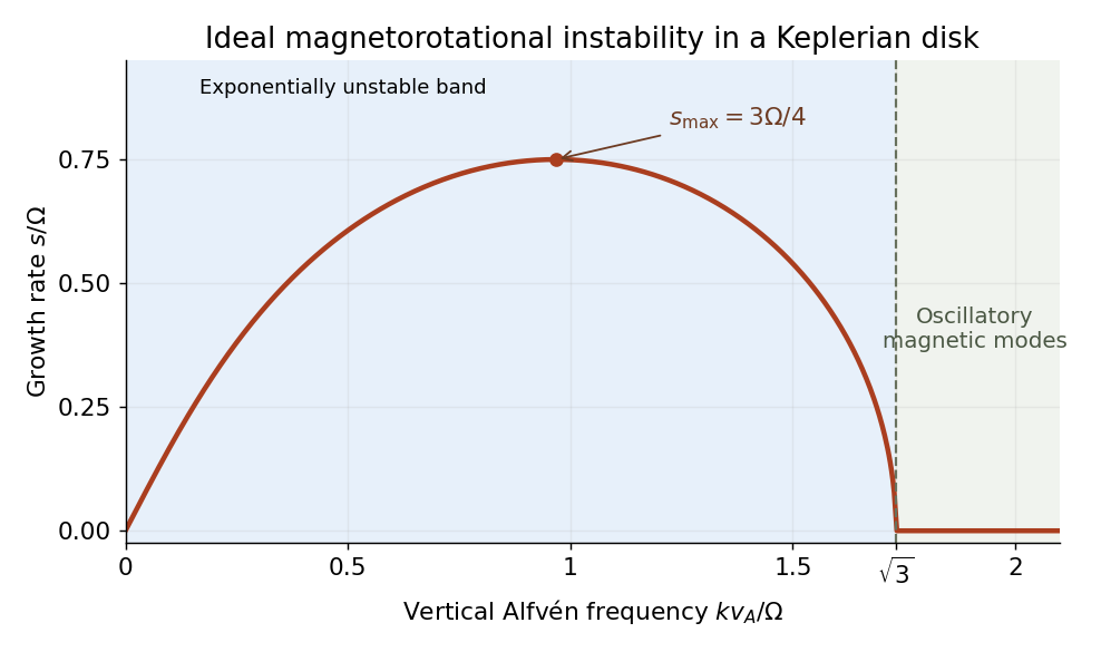
Work locally at with , and defineHere is the radial epicyclic frequency. Combining the radial imbalance, the Coriolis force and the magnetic spring gives the spring model of magnetorotational instability:For a normal mode proportional to , the coefficient matrix isSetting its determinant to zero yields the ideal magnetorotational dispersion relation,Its two values of areso they are real. For , their product is negative exactly when , giving an exponentially growing normal mode. Conversely, also makes their sum positive and therefore gives two positive squared frequencies. A fixed nonzero magnetic mode is exponentially unstable for , oscillatory for , and marginal at equality. Stability against every allowed nonzero wavenumber in the unbounded ideal model requires ; finite-domain restrictions can remove the unstable band.
For , the equilibrium relation gives , so and . Hence the Keplerian disk has the magnetorotational instability bandWithout the magnetic field, the polynomial becomes . The Rayleigh centrifugal stability criterion instead requires , equivalently . A Keplerian disk satisfies that hydrodynamic criterion. Magnetic coupling therefore destabilizes a disk that has a restoring hydrodynamic epicyclic oscillation; the field couples angular-momentum exchange between elements, rather than acting only as an isolated restoring spring.
Using the given linear momentum balance, multiply by the velocity and integrate over the fixed volume:This is integration by parts component by component, or the divergence theorem. The first term is boundary stress power. With component-first velocity gradient , the second is the double contraction .
For a Newtonian fluid, , where is the rate-of-strain tensor and is dynamic viscosity. Incompressibility removes the pressure contribution, and the symmetric tensor is orthogonal to the antisymmetric part of . ThereforeThe displayed energy identity follows for the stated linear balance. A full advective momentum equation in a fixed control volume would also contribute an advective kinetic energy flux. The nonnegativity statement here is for a purely Newtonian viscous stress; a viscoelastic stress can exchange stored free energy with the flow.
Let , , and . The configuration equation of the Hookean dumbbell model becomesHere the paper's denotes the Boltzmann constant . Integrating the second moment equation against and discarding boundary terms at infinite separation givesFor example the spring drift differentiates each factor , while the Laplacian gives . The Hookean dumbbell conformation equation isIn the row-vector convention of , the displayed gradient tensor is , giving exactly the transposes in the requested equation. The dimensionless conformation tensor consequently has upper-convected derivative , with polymer relaxation time . This normalization matters: the unscaled has equilibrium value , rather than .
Write the centre position as and the bead positions as . In the affine velocity field, . The midpoint follows the flow, so its two slip velocities areEach bead loses mechanical power times its squared slip speed. Adding the two powers proves the drag dissipation of a bead-spring pair:The factor one half comes from two equal-and-opposite bead slips, not from assigning only one bead a drag force.
The claimed equality does not hold for the printed joint distribution. The original PDF specifies a centered Maxwell-Boltzmann distribution of independent of , withSince the double average includes number density , evaluating the Gaussian integrals givesThe cross term vanishes because the conditional mean of is zero. In particular, set and take the equilibrium configuration probability density . The left side is , while . This is a counterexample even at thermal equilibrium, so no rearrangement of the earlier conformation tensor equation can prove the printed statement.
The discrepancy is thermal bead drag and heat-bath power: gross viscous loss of microscopic thermal motion is replenished by the thermal bath. It is not identical to mechanical polymer stress power. Moreover, in the earlier configuration continuity equation is a probability current velocity, including a distribution-dependent osmotic drift; it cannot simultaneously be identified with an independently sampled centered Maxwellian velocity.
A consistent overdamped result is the free-energy balance of a Hookean dumbbell. Define andDifferentiate the relative entropy and use the configuration Fokker-Planck probability current . After integration by parts,The affine osmotic term is . HenceThe polymer stress tensor has in an incompressible flow. It stores or releases free energy as well as dissipating it, so the total stress-work term in part a need not itself be a purely dissipative quantity for this viscoelastic material. Stress power equals only for stationary free energy, and uses the probability-current slip. Neither condition turns the printed independent-Maxwellian average into that expression.
Solutions to both questions and all eight parts. The diffusion coefficient and the amplitude-versus-energy damping convention are stated explicitly; the final rotation calculation uses the supplied isolated-sphere incident flow.
Take the inviscid limit of the Navier-Stokes equation, neglect gravity, and use ideal magnetohydrodynamics. The governing equations areThe continuity equation also gives . Write the first-order magnetic perturbation as and linearize about the uniform stationary background:For a nonzero-wavenumber plane wave proportional to , the two divergence constraints imply . The longitudinal momentum equation then gives for that mode, and gives for nonzero . Thus the propagating Alfvén wave is transverse. Its two independent transverse directions have the same dispersion relation.
The Linear Alfvén wave equations reduce toEliminating either amplitude givesFor , the branch traveling along has and . The opposite branch reverses that amplitude sign. Finite viscosity would additionally damp the motion; it is neglected in obtaining the real ideal dispersion relation.
Subtract the constant equilibrium magnetic energy density. Since , the perturbation densities areThe traveling-wave amplitude relation from part a givesThis is pointwise Alfvén wave energy transport for one traveling wave, not a claim that every superposition or standing wave has pointwise equipartition.
For the real fields written as and similarly for , the period averages areThe factors one half distinguish a sinusoid's peak amplitude from its mean squared value; the same complex-vector convention also covers circular polarization of waves.
In ideal magnetohydrodynamics, the first-order electric field is . Retaining its product with both the background and first-order magnetic field gives the Poynting vectorThe first term is transverse and oscillatory, with zero period average. The second is quadratic and transports wave energy. A potential quadratic ideal electric-field term vanishes here because the real traveling-wave fields are parallel or antiparallel.
For the branch, , soFor the opposite branch, its sign reverses. The averaged Poynting flux is the total wave energy density, including equal kinetic and magnetic shares, multiplied by the group velocity. This agrees with Alfvén wave energy transport. Although the flux in this expression is electromagnetic, it supplies the transport of both components of the coupled fluid-field wave.
In this question, the coefficient multiplying is the magnetic diffusivity. Denote it ; it is the paper's , with dimensions of length squared per time. If denotes electrical resistivity, then . The two conventions must not be interchanged.
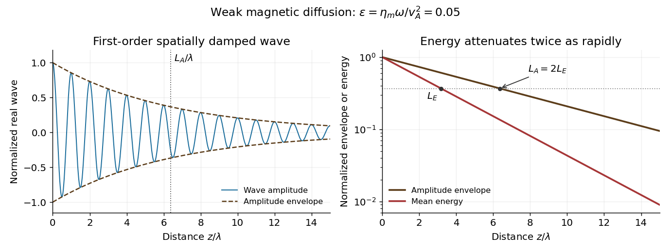
For an imposed real positive , retain the momentum equation and useElimination gives the exact Resistive damping of an Alfvén wave relationHere is complex because the driving frequency is real. Introduce the dimensionless diffusion parameter . For propagation and attenuation along , choose the square-root branch with . The spatial damping of a driven Alfvén wave isWith the convention , the amplitude decays as . Define its e-folding length and the wavelength . ThenIf damping length instead refers to wave energy, the squared amplitude decays twice as fast: and . Stating the convention avoids a factor-of-two ambiguity. The temporal damping rate at fixed real is a different specification from this imposed-frequency problem.
Expand the given translating-sphere Stokes flow into its Stokeslet and potential dipole parts:The second parenthesis is and has zero curl outside the sphere. For the first,Thus the vorticity of translating-sphere Stokes flow isThe result is independent of the irrotational finite-size dipole correction. It holds in the exterior ; the singular solid harmonics are used only outside their source.
Use the force flux at infinity in Stokes flow. With an outward normal from a large sphere, the force on the body is . Let . The leading far-field velocity and pressure areTheir rate-of-strain tensor isIn the Newtonian fluid stress tensor , the isotropic pieces cancel. Consequently,The second spherical moment integral follows from rotational symmetry and . Since , taking gives the Stokes drag law:The omitted dipole contributes a surface integral of order and vanishes in this limit. The sign refers to the fluid's drag on the moving sphere.
At the terminal velocity, buoyancy-corrected weight balances the Stokes drag law:HenceA denser sphere falls in the direction of ; a lighter one rises. Equal densities give no sedimentation. The calculation assumes negligible fluid Reynolds number, an unbounded fluid, and negligible transient body acceleration after terminal settling. The fluid mass density enters through buoyancy and through the small-Reynolds number condition.
Take positive upward, let sphere A's centre be , and write its downward velocity as , with . At B's centre the displacement from A is . The vorticity of translating-sphere Stokes flow therefore givesB is held in translation but has zero applied torque. By Faxén's rotational law, it rotates with half the incident vorticity:Integrating the rotation induced by a passing Stokes sphere along the complete path cancels :Its magnitude is radians, with direction about the negative axis by the right-hand rule. All instantaneous rotations have this same axis, so the integrated angular velocity gives the net angle without a noncommuting-rotation correction. The result is independent of B's radius in the prescribed incident-flow calculation.
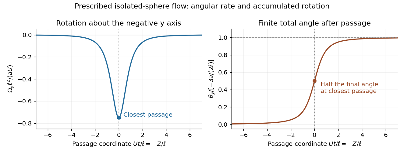


The inequality ensures no overlap. It does not by itself make mutual hydrodynamic interactions negligible: the stated flow is the isolated-A solution, and a held finite B also disturbs A's flow. Thus the displayed angle is the result for that supplied incident flow, or the leading one-way approximation to separated bodies. A fully coupled two-sphere calculation uses the method of reflections for Stokes flow or an exact pair resistance solution.
Write the physical magnetic field as and use the constant mass density to introduce Alfvén velocity units, . If is the fluid's mechanical pressure, the magnetohydrodynamic total pressure per unit mass density is . The ideal magnetohydrodynamic equations then reduce toThe first equation is momentum conservation: the magnetic pressure has been included in , leaving magnetic tension explicitly. The second is the ideal magnetohydrodynamic induction equation, expressing magnetic flux freezing. The last two equations impose incompressibility and the solenoidal magnetic-field constraint.
The model assumes a smooth conducting-fluid continuum with constant mass density and constant magnetic permeability, nonrelativistic velocity, and scales on which a single-fluid description is appropriate. Negligible electrical resistivity removes magnetic diffusion; negligible viscosity removes viscous momentum diffusion. Equivalently, the magnetic Reynolds number and the Reynolds number are large on the scales being retained. The low-frequency approximation neglects the displacement current; Hall and other kinetic corrections to Ohm's law are absent. Incompressibility is an imposed approximation, commonly justified when the Mach number is small. There is no independently evolved thermodynamic pressure: enforces the incompressibility condition. We omit external body forces; a conservative one could instead be absorbed into .
The magnetic second-moment tensor is . This is the magnetic dyadic called the Maxwell tensor in the paper; the isotropic part of the usual Maxwell stress tensor is already contained in the magnetohydrodynamic total pressure. The solenoidal magnetic-field constraint givesConsequently the magnetohydrodynamic momentum equation in part a becomes , where is the material derivative. Applying its product rule and the ideal magnetohydrodynamic induction equation givesThus the evolution uses only , together with . To determine , take the divergence of the magnetohydrodynamic momentum equation. Since and ,This is the pressure Poisson equation for incompressible flow, with boundary conditions supplied by the imposed normal acceleration and normal stress, or by periodicity or decay at infinity as appropriate. For example, the normal component of the magnetohydrodynamic momentum equation requires at a prescribed boundary. The pressure is determined up to a spatially constant function of time.
For equivalence to one resolved magnetic field, the initial must actually be for a divergence-free vector field. In particular it is a symmetric positive semidefinite matrix of matrix rank at most one. The tensor equations also admit more general stresses; the averaged in part d need not have matrix rank one.
With zero velocity and no time dependence, the magnetic second-moment tensor equation holds automatically, but the magnetohydrodynamic momentum equation still requiresThe magnetic tension must therefore be a pressure gradient. Locally, its necessary integrability condition ison a simply connected region this is also sufficient for a scalar , subject to the global boundary conditions. In physical units the same balance is : the Lorentz force density is balanced by mechanical pressure, rather than necessarily vanishing. A zero mean magnetic field does not make the local magnetic tension zero, so an arbitrary tangle is not automatically a static equilibrium.
Take the trace of the statistically isotropic magnetic second-moment tensor. There are three spatial directions, soChoosing the nonnegative speed,Thus is the root-mean-square value of any one Cartesian magnetic field component in Alfvén velocity units. It is not the magnitude of the mean Alfvén velocity, which is zero here. Statistical isotropy fixes a second moment even when the first moment vanishes.
Average the equations in part b and make exactly the prescribed scale-separation approximation: the retained perturbations vary on lengths much greater than , and perturbations at the tangle scale are omitted. Products of two retained perturbations can then be neglected. Writing , and , the linearized equations areNo unmodelled small-scale response has been inserted into this closure.
Introduce the fluid displacement by and choose . Integrating the magnetic second-moment tensor equation giveswhere is a time-independent integration tensor set by the initial stress. For a pure oscillatory normal mode, . Its restoring force is therefore : the isotropic magnetic tangle has the same transverse response as an incompressible elastic medium with shear modulus .
For a plane wave proportional to , with , incompressibility gives . The tensor equation and magnetohydrodynamic momentum equation becomeDotting the second equation with yields for , since . Substitution then givesThere are two independent transverse polarizations. The phase speed is in every direction, and the two signs of give group velocities . These magnetoelastic waves in an isotropic magnetic tangle exist because a shear deformation distorts the second moment of the tangled magnetic field, producing a restoring magnetic tension even though its mean is zero.
For comparison, a uniform magnetic field with Alfvén velocity gives the incompressible Alfvén wave relation . Its frequency depends on the direction of , and energy propagates along . Here the averaged restoring response is isotropic: there is no preferred mean-field direction. Both systems resist transverse deformation through magnetic tension, rather than through compressive sound.
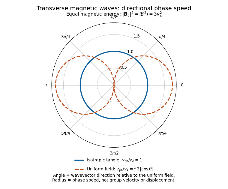
Directional phase speeds for a magnetic tangle and a uniform magnetic field with the same mean-square strength
. The radial coordinate is phase speed divided by the tangle wave speed. The circular tangle curve is direction independent; the uniform-field curve is proportional to the absolute cosine of the propagation angle. These are phase-speed curves, not group-velocity trajectories. Details.
The propagating branch is not the entire perturbation space. For example, , and solve the linearized equations without propagation, for any small, slowly varying . Such a static stress perturbation in magnetoelastic wave equations balances a pressure gradient. Thus the requested wave conclusion applies to the oscillatory branch; it must not exclude stationary initial stress perturbations.
The common part of the magnetohydrodynamic-viscoelastic analogy is stretching and advection of a line element. With the component-first velocity gradient , the ideal tensor equation isIts left side is an upper-convected derivative, the same deformation law that appears for a polymer conformation tensor when its relaxation is neglected.
There are two important physical differences. First, the solenoidal magnetic-field constraint prevents a magnetic field line from having an isolated source or sink inside the fluid. A polymer strand can have molecular endpoints, so there is no corresponding no-endpoint constraint on the strands. Second, a stretched polymer has a preferred relaxed distribution of configurations and a finite polymer relaxation time; it can recoil relative to the solvent through molecular drag and thermal motion. An ideal magnetic field has no analogous local tendency to return to a prescribed coil size. Real polymers also have a finite contour length, a limitation absent from the ideal field-stretching law.
For example, a normalized Hookean dumbbell conformation equation has the dissipative extensionThis is local relaxation toward an isotropic thermal configuration. It remains nonzero for a spatially uniform stretched . By contrast, constant magnetic diffusivity adds to the resistive induction equation. The product rule gives the resistive evolution of the magnetic second-moment tensor:The magnetic correction involves spatial gradients, vanishes for a uniform magnetic field, and does not create field-line endpoints: . It permits slippage and magnetic reconnection while preserving the no-monopole constraint. After averaging, its gradient-product term generally needs additional information beyond the averaged . One cannot replace it indiscriminately by the local polymer relaxation term, or even by alone.
Work in the laboratory frame, with the fluid at rest at infinity. SetAt , and , so the no-slip boundary condition is on the translating sphere. As , and the gauge-fixed pressure tends to zero.
It is also possible to check the exterior Stokes equations directly. Differentiating the radial functions givesandThus the Newtonian fluid stress tensor satisfies throughout .
Let point away from the common centre on each concentric sphere. Applying the divergence theorem to the intervening fluid shell, whose inner normal is , yieldsThis is the force flux at infinity in Stokes flow. It is legitimate even though the stress tensor tends to zero pointwise, because the area of the large sphere grows as .
For an explicit evaluation, put and . The leading terms are and . Their velocity gradient isAfter symmetrizing and subtracting the pressure contribution,By rotational symmetry, . HenceThis is Stokes's law, with the force on the sphere opposite its velocity. For a component calculation with , the same integral is .
Neglect the inertia of the sphere and balance the applied force against Stokes drag. The sphere translates with , where . The applied force is also the net force transmitted to the fluid; the fluid's drag on the sphere has the opposite sign.
Translate the origin to . In the solution of part a, retain the terms of order and discard those of order . With ,This is the Stokeslet, or equivalently the Oseen tensor acting on . The omitted finite-size velocity is of order , so the displayed term is the leading far field for . The singular Stokeslet must not be evaluated at its own centre to obtain a particle's self mobility.
Use the deterministic Hookean dumbbell model, with a zero-rest-length spring and negligible connector drag. For , its elastic forces on the two beads areHere is the spring constant. No independent thermal forcing from Brownian motion or bead inertia is included. The unperturbed linear velocity field is , with by incompressibility.
The fluid velocity used in each bead's drag law is the imposed flow plus the disturbance from the other bead, with its own singular field omitted. At leading order in , the evenness of the Oseen tensor, , givesThese are the pair hydrodynamic mobility matrix relations. Their signs follow from balancing each spring force with , the fluid drag on that bead.
Adding the equations cancels both the direct spring slips and the cross-induced velocities, since . For the midpoint ,The midpoint therefore follows the undisturbed linear velocity field. Subtracting the equations instead gives the hydrodynamic interaction of a Hookean dumbbell:The dimensionless interaction matrix isIts transverse and longitudinal eigenvalues are and , respectively. Since the spring force is longitudinal, the separation equation can also be writtenThe relative correction to the free-draining spring relaxation rate is therefore , explicitly proportional to . Entrainment by the other bead reduces their relative approach for given opposing spring forces.
This is a far-field hydrodynamic interaction, valid for ; it is not a near-contact law and omits higher reflections and lubrication. The printed target also fixes the spring's rest length implicitly. For an ordinary spring obeying Hooke's law with nonzero rest length , the elastic force would be , and every spring term above would acquire the factor . The displayed result uses the zero-rest-length spring convention appropriate to the ideal Hookean dumbbell model.
Let and be the complex plane wave amplitudes and set , . The linearized Euler equations in the rotating frame areHere is pressure per unit mass density, including the centrifugal potential. The last line is incompressibility, not an additional equation of state.
Taking the curl eliminates pressure. For constant and a divergence-free vector field, . Thus the inertial-wave vorticity equation givesApply once more and use . For a nonzero oscillatory amplitude,so the inertial-wave dispersion relation isThe restoring influence is the Coriolis acceleration. In particular . For , the projected linear dynamics have zero frequency; these are steady balanced disturbances rather than the nonzero-frequency branch used in the division above. The spatially uniform mode must be treated separately from this dispersion relation.
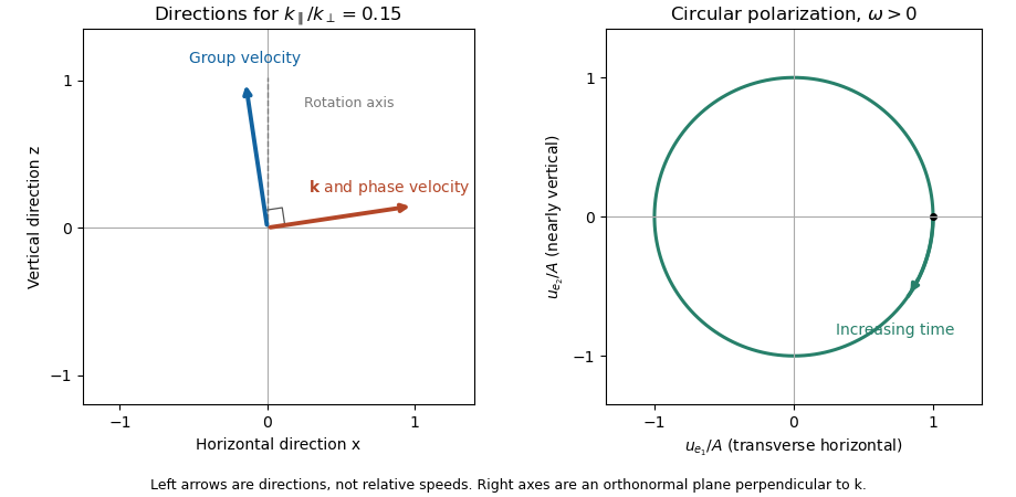
The group velocity, which gives wave-packet and energy propagation, is the gradient of the dispersion relation:For this becomesThus for , energy travels almost along the rotation axis, with a small horizontal component. By contrast, the normal-to-phase-front phase velocity is almost horizontal. Indeed , so these phase and group directions are perpendicular. Specifying which meaning of propagation is intended matters for an inertial wave.
For the wave polarization, incompressibility and the equation in part a giveThe horizontal component parallel to is small, but : the other horizontal and vertical components are in quadrature. More exactly, introduce the orthonormal transverse basisThen . The physical velocity at a fixed point traces a circle in the plane perpendicular to ; its handedness reverses between branches. In the anisotropic limit this plane is nearly vertical. The group velocity and polarization of an inertial wave therefore have quite different geometric roles.

Let and let be the common size of horizontal and vertical velocity perturbations, as found in part b. The linear inertial wave time and nonlinear advection time areThe critical balance in a rapidly rotating fluid is thereforeThe Rossby number is of order . Horizontal geostrophic flow balances the leading pressure gradient against Coriolis acceleration, soThese are dimensionally comparable statements, rather than comparisons of a dimensional frequency with a dimensional velocity. Equivalently, use and as units. ThenThus rotation stays in these units, while the motions evolve on the slower time. Vertical advection is smaller than horizontal advection by .
Write , with , and . At leading horizontal order,Define the stream function , including its horizontally uniform part in this convention. ThenThe next-order incompressibility condition is not zero horizontal divergence:This term has size and is essential: its product with the large rotation rate is a leading contribution to the vertical vorticity equation.
To see that contribution explicitly, write . At the first horizontal inertial order,Taking its vertical curl eliminates . The two-dimensional advection identity and the two divergence orders giveEquivalently the ageostrophic flow satisfieswhose divergence is . This explicitly verifies that the next-order divergence has the required sign.
The vertical momentum equation, at the same slow order, isFinally , where the canonical two-dimensional Poisson bracket is . The reduced equations for an anisotropic rotating fluid areThe omitted vertical-advection, ageostrophic-advection and relative-vorticity stretching terms are smaller by in the equations retained here. Linearizing these equations recovers , the anisotropic limit of part a.
Within the reduced equations for an anisotropic rotating fluid, a flow that remains purely horizontal has and . The second reduced equation therefore requiresThus the retained horizontal motion is two-dimensional. This is a Taylor–Proudman theorem consequence in the slow balanced ordering; setting at only one instant would not suffice, because vertical motion could subsequently develop.
The word “exactly” applies to the reduced model. It is not a theorem for every finite-Rossby number solution satisfying only . For example, the full rotating Euler equation admitsIt is an incompressible flow, has zero nonlinear advection, and obeys . It is purely horizontal but depends on , and can hold. This fast inertial oscillation lies outside the slow anisotropic critical balance used in part c; it shows why that ordering cannot be dropped from the conclusion.
For a uniform axial magnetic field, the anisotropic Shear Alfvén wave is predominantly horizontally polarized, whereas the pseudo-Alfvén wave is predominantly vertically polarized. Without rotation both have characteristic frequency . Pressure projection makes the effective Coriolis acceleration couple these two transverse wave polarization states at the inertial-wave rateThus the useful comparison is not alone, nor anisotropy alone, butIn this limit rotational coupling of shear and pseudo-Alfvén waves is negligible on an Alfvén propagation time, so the two familiar linear polarizations are decoupled to leading order. The factor cancels: simply making both disturbances more anisotropic does not by itself remove their relative rotational coupling.
For a nonlinear reduction one must also make the rotational mixing slow compared with the nonlinear evolution being retained. Under Alfvénic critical balance, , the same inequality gives . Rapid rotation relative to the horizontal nonlinear rate can therefore coexist with leading Alfvénic decoupling in the windowHigh electrical conductivity makes magnetic diffusion slow, and the corresponding inviscid approximation is also assumed. If , rotational and magnetic restoring effects are comparable and the modes are mixed magneto-Coriolis disturbances; in the rotation-dominated limit they separate into fast inertial-like and slow magnetostrophic branches, rather than into independently evolving shear and pseudo-Alfvén polarizations.
At finite amplitude, independence is generally one-way in the usual anisotropic ideal magnetohydrodynamics reduction: the Alfvénic subsystem has no leading feedback from pseudo-Alfvénic perturbations, but it can still advect them. The small rotational-coupling condition removes an additional two-way coupling, rather than all nonlinear advection.
This is an asymptotic finite-timescale statement. The two nonrotating Alfvén polarizations are degenerate, so even a weak nonzero rotational coupling can rotate their superposition over the much longer time . Exact decoupling for arbitrarily long times does not follow from a small ratio alone. The strictly nonpropagating limit is separate.
Use the same constant dynamic viscosity for both incompressible Stokes flows, and let be body force per unit volume. Their equations and Newtonian fluid stress tensor arewhere is the strain-rate tensor. Consider the cross-work fluxBy the product rule,The pressure terms vanish by incompressibility. Symmetry of the stress tensor removes antisymmetric velocity gradient contributions, leaving in both cross terms; they cancel. Apply the divergence theorem, with outward from , and rearrange:This is the Lorentz reciprocal theorem with body forces. It depends on reciprocal linear viscous response in the same fluid; arbitrary unrelated constitutive laws would not supply the cross-term cancellation.
Write the supplied velocity in the radial formAt , and , giving the no-slip boundary condition . At infinity and the supplied gauge-fixed pressure tends to zero. These are the laboratory-frame conditions for a sphere translating through otherwise quiescent fluid.
The exterior Stokes equations can also be checked directly:andTo compute surface traction in translating-sphere Stokes flow, let point from the sphere into the fluid. At the surface, , and . HenceSubstitute into the Newtonian fluid stress tensor. Its viscous contribution to the surface traction is , so the normal part cancels the pressure contribution:The vector is constant over the entire sphere in the stated pressure gauge. Integrating it gives the fluid's drag force on the sphere,This is Stokes's law. On an exterior fluid domain the outward domain normal at its inner boundary is ; that distinction will matter in the reciprocal calculation.
Articles were limited to the first 100 out of 146 total.
Articles by others on the same topic
There are currently no matching articles.