Past exam of the algebra 1 and differential equations 1 course of the University of Oxford / 2014 / 6

Use the Fourier transform conventionThe absolute integrability of $v$ makes this integral exist for every real $\omega$, with $|\hat{v}(\omega )|\le \Vert v{\Vert }_1$. With this convention the inverse Fourier transform has factor $1/(2\pi )$; maintaining that normalization is essential in part (e).

The profile is an even function, so its Fourier transform is real andFor $\omega \ne 0$, integration by parts givesThereforeAt zero, direct integration gives the area of the triangle, namely two; the displayed quotient has the same limit. In particular $\hat{T}(\omega )\ge 0$ for every real frequency. This is the Fourier transform of a triangular function.

One can also see the nonnegative square structurally: $T=\frac{1}{2}{1}_{[-1,1]}\ast 1_{[-1,1]}$, so the convolution theorem gives $\hat{T}=\frac{1}{2}(2\sin \omega /\omega {)}^2$.

Complete the square inside the Fourier transform of the Gaussian heat kernel:After $z=x/(2\sqrt{t})$,The supplied shifted Gaussian integral equals $\sqrt{\pi }$ for real $\sqrt{t}\omega$. HenceAt zero this says $\int q_t=1$, so convolution with the heat kernel averages rather than rescales the initial mass. The formula is an instance of the Fourier transform of a Gaussian.

Both kernels are integrable functions, so the convolution theorem givesThe uniqueness of the Fourier transform on integrable functions gives equality almost everywhere. Both sides are continuous, so it holds at every point:For completeness, continuity of the convolution follows by dominated convergence: $q_t$ is bounded and continuous, so for $x_j\to x$ the integrands $q_t(x_j-y)q_s(y)$ converge pointwise and are dominated by $\Vert q_t{\Vert }_{\infty }{q}_s(y)$.

The identity is the heat semigroup property: evolving for time $s$, then for time $t$, is the same as evolving once for time $s+t$.

For fixed frequency $\omega$, the Fourier transform of a derivative gives $\widehat{u_{xx}}=-{\omega }^2\hat{u}$. The transformed initial value problem is thereforeSolving this scalar ordinary differential equation yieldswhere the value at $\omega =0$ is interpreted by continuity and equals two. Thus diffusion suppresses high frequencies by the Gaussian multiplier while preserving the zero-frequency mass.

The differentiation and transform steps are justified for the heat kernel solution $u=q_t\ast T$: for positive time its spatial derivatives are integrable, since Gaussian derivatives are integrable and $T$ is bounded with compact support. Alternatively, the transformed calculation first suggests the formula, and the next part verifies the resulting solution directly.

Insert part (i) in the inverse Fourier transform. The factor two in $\hat{T}$ cancels half of the inverse normalization:The integrand has a removable singularity at zero. For $t>0$, the Gaussian controls every polynomial factor at infinity, so differentiation under the integral is valid. Differentiation in $t$ and twice in $x$ both multiply the integrand by $-{\omega }^2$, proving $u_t=u_{xx}$.

There is also a direct physical-space representation:Since $q_t$ has integral one, writeThe continuous compactly supported profile $T$ is uniformly continuous. Given $ϵ>0$, choose $\delta >0$ so its change is below $ϵ$ for $|y|<\delta$. That part of the integral is bounded by $ϵ$. The other part is bounded by $2\Vert T{\Vert }_{\infty }{\int }_{|y|\ge \delta }{q}_t(y)dy$, which tends to zero by the substitution $y=2\sqrt{t}z$ and the vanishing tails of the Gaussian integral. This proves $u(t,x)\to T(x)$ uniformly as $t\downarrow 0$ and verifies the initial condition.

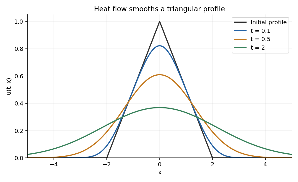
Thus the formula supplies the full heat evolution of a triangular profile, including the corner points of the initial profile. Positive time immediately smooths those corners.