Past exam of the algebra 1 and differential equations 1 course of the University of Oxford / 2014 (A1, 4320)

Source release: Oxford examination archive, member FOI-20210708-1 - Data/4320.pdf. The cover dates this examination to 18 June 2014, 2.30–5.30pm. The six questions have 36 leaf parts, answered in source order below.

The minimal polynomial $m_T$ is the monic polynomial of least polynomial degree such that $m_T(T)=0$. Here a polynomial $p(x)={\sum }_j{c}_j{x}^j$ is evaluated at the linear operator by $p(T)={\sum }_j{c}_j{T}^j$, with the constant term acting as $c_{0}I$.

An annihilating polynomial exists because $I,T,T^2,\dots$ lie in the finite-dimensional vector space ${\mathrm{End}}_F(V)$ and are therefore eventually linearly dependent. Uniqueness follows by subtracting two monic annihilators of the same least degree: their difference has smaller degree and still annihilates $T$.

Equivalently,For the forward implication evaluate the factorization at $T$. For the reverse implication divide $p$ by $m_T$ using polynomial division; the remainder annihilates $T$, so minimality makes it zero. This also identifies the annihilating polynomials as the principal ideal generated by $m_T$.

Suppose $E^2=E$. Every vector has the decompositionIf $w=Ez$ also belongs to $\ker E$, then $w=E^{2}z=Ew=0$. HenceOn its image of a linear map, $E$ acts as the identity; on its kernel of a linear map, it acts as zero. Concatenate a basis of the image with a basis of the kernel. The resulting matrix is $\mathrm{diag}(I_r,0)$, where $r=\mathrm{rank}E$.

Conversely, this block matrix squares to itself, so any linear map having that matrix in a basis satisfies $E^2=E$. Thus projection operators are precisely the linear maps with this block form. This is an algebraic projection; no inner product or orthogonality is required.

Evaluate Bézout's identity for polynomials at $T$:All these linear operators commute because they are polynomials in the same operator. Thus every $v\in V$ can be writtenThe first summand belongs to $\ker p(T)$ and the second to $\ker q(T)$, since applying the corresponding operator introduces the product $p(T)q(T)=0$.

If $v$ lies in both kernels, the same identity gives $v=0+0=0$. Therefore the sum is direct:This is the kernel decomposition for coprime polynomials. It uses both annihilation by $pq$ and the coprimality expressed by the Bézout identity.

Write $U=\ker p(T)$, $W=\ker q(T)$. The linear operator $E=a(T)p(T)$ vanishes on $U$. On $W$, the identity $E=I-b(T)q(T)$ gives $Ew=w$.

By the direct sum in part (i), every vector has a unique expression $u+w$, andConsequentlyThe complementary projection operator is $I-E=b(T)q(T)$, onto $U$ along $W$. These are polynomial projections for a coprime decomposition. In particular the projection does not depend on which Bézout coefficients are chosen: its action on the two summands uniquely determines it.

Let $P=b(T)q(T)$ and $Q=a(T)p(T)$. By part (ii), these are complementary projection operators with images $U=\ker (T-\lambda I{)}^{\alpha }$ and $W=\ker (T-\mu I{)}^{\beta }$. Thus $D=\lambda P+\mu Q$ acts as $\lambda I$ on $U$ and $\mu I$ on $W$.

The linear operator $T$ preserves both summands because it commutes with its own polynomials. Therefore $N=T-D$ preserves them too, and its restrictions satisfyPut $k=\max (\alpha ,\beta )$. Both restrictions of $N^k$ vanish, so the direct sum givesHence $T-D$ is a nilpotent linear map. The operator $D$ is diagonalizable, since its two summands are its eigenspaces, and it commutes with $T$. This illustrates the Jordan–Chevalley decomposition in the case of two distinct eigenvalues.

Choose a basis and let $A$ be the matrix of $T$. Use the monic conventionUnder a change of basis, $A$ becomes $B=P^{-1}AP$ for an invertible matrix $P$. Thenso multiplicativity of the determinant gives $\det (xI-B)=\det (xI-A)$. Therefore the characteristic polynomial is independent of the chosen basis and is well-defined for the linear transformation itself.

The given $J$ satisfies $J^2=-I_{2m}$ and is invertible. Taking determinants in the defining identity of a symplectic matrix givesSince $\det (M^T)=\det M$ and $\det J\ne 0$, cancellation yields $(\det M{)}^2=1$. HenceIn particular every symplectic matrix is invertible. This argument establishes the requested alternatives; the later parts explicitly supply the determinant-one hypothesis that they use.

The identity is symplectic because $I^{T}JI=J$. For two symplectic matrices $M,N$,Thus the set is closed under matrix multiplication. Every member is invertible by part (i). Multiplying $M^{T}JM=J$ on the left by $M^{-T}$ and on the right by $M^{-1}$ givesso it is also closed under inverses. Associativity is inherited from the general linear group. These facts prove that the symplectic group is a subgroup of $\mathrm{GL}(2m,\mathbb{R})$.

Rearrange $M^{T}JM=J$ asThus $M^{-1}$ is similar to $M^T$. Similar matrices have the same characteristic polynomial by part (a), and transposition also preserves it:Therefore $\boxed{{\chi }_{M^{-1}}={\chi }_M}$. This is the underlying algebraic source of the reciprocal spectrum of a symplectic matrix.

For $\lambda \ne 0$, factor the matrix inside the determinant:The second line uses $\det M=1$; the third uses the even matrix size; the last uses part (i). ConsequentlyIn other words, the characteristic polynomial equals its reciprocal polynomial.

Let $P={\chi }_M$, and suppose $P(z)=(z-\lambda {)}^{d}R(z)$ with $R(\lambda )\ne 0$. The reciprocal identity gives, for $x\ne 0$,Near $x={\lambda }^{-1}$ the factor $x^{2m-d}R(1/x)$ is nonzero. Also $1-\lambda x=-\lambda (x-{\lambda }^{-1})$ has a simple zero there. HenceThis proves equality of the algebraic multiplicities, not merely that the inverse is another eigenvalue. Invertibility excludes zero eigenvalues throughout.

The fixed points of reciprocal root pairing are $1$ and $-1$, so part (iii) alone does not establish their parity. Use the polynomial identity itself.

Write $P(x)=(x-1{)}^{r}A(x)$, where $A(1)\ne 0$ and allow $r=0$ if one is not a root. After substituting in $P(x)=x^{2m}P(1/x)$ and canceling $(x-1{)}^r$ away from $x=1$, obtainLetting $x\to 1$ yields $A(1)=(-1{)}^{r}A(1)$, so $r$ is even.

Similarly write $P(x)=(x+1{)}^{s}B(x)$ with $B(-1)\ne 0$. This time cancellation gives $B(x)=x^{2m-s}B(1/x)$. Letting $x\to -1$ yields $B(-1)=(-1{)}^{2m-s}B(-1)$, so $s$ is even. ThusThe conclusion includes multiplicity zero. It is a consequence of the reciprocal identity in even degree, which is stronger at these fixed points than just pairing the roots.

The rank-nullity theorem states that for a linear map $A:X\to Y$ with finite-dimensional domain,Equivalently, nullity plus rank equals the dimension of the domain. One proof extends a basis of $\ker A$ to a basis of $X$; the images of the added vectors form a basis of $\mathrm{im}A$.

The annihilator of a vector subspace $W\le V^{\ast }$ isIf $\dim W=k$, extend a basis of $W$ to one of $V^{\ast }$. In the resulting dual basis of $V^{\ast \ast }$, the last $n-k$ coordinate functionals span $W^{\circ }$. Hence $\boxed{\dim W+\dim W^{\circ }=n}$.

The bidual evaluation map $j:V\to V^{\ast \ast }$ is $j(x)(\varphi )=\varphi (x)$. It is a linear isomorphism in finite dimension. Its inverse image of the annihilator isThis identification uses evaluation only; no choice of inner product is involved.

Under the bidual evaluation map, a vector $y$ lies in $(\mathrm{im}\Phi {|}_U{)}^{\circ }$ exactly whenThat is precisely membership of the orthogonal complement for a bilinear form. ThereforeThe dimension formula in part (ii) givesso $\boxed{\dim U+\dim U^{\perp }\ge n}$. More precisely, the rank-nullity theorem givesThis is the orthogonal complement dimension for a degenerate bilinear form. The possible excess comes from vectors annihilated by the form against all of $V$.

The dimension formula for a sum of subspaces and the zero intersection implyBut $U+U^{\perp }$ is a vector subspace of the $n$-dimensional space $V$, so its dimension is at most $n$. Equality follows, and the sum is all of $V$. Since the intersection is zero, it is a direct sum:The argument remains valid for a degenerate ambient symmetric bilinear form; it uses the stated intersection hypothesis rather than assuming nondegeneracy everywhere.

Use the $m$-dimensional space $V_m$ for this change of basis. With the columns of $P$ recording the new basis in the old one, bilinearity givesThus the matrices of the bilinear form satisfyThis is matrix congruence, rather than the similarity rule for an endomorphism: both arguments of the bilinear form change basis.

The restriction of a positive definite form to each $V_m$ is positive definite. By the spectral theorem for real symmetric matrices, choose an orthogonal matrix $P$ such that $P^T{A}_{m}P=\mathrm{diag}(d_1,\dots ,d_m)$.

Each $d_i=\phi (f_i,f_i)>0$, since a basis vector is nonzero. Taking determinants in part (i) givesbecause an orthogonal matrix has determinant $\pm 1$. ConsequentlyThese determinants are the leading principal minors in Sylvester's criterion.

Work inside $V_{m+1}$, and take the orthogonal complement for a bilinear form of $U=V_m$ relative to this ambient space. If $z\in U\cap U^{\perp }$, then $\phi (z,z)=0$, so positive definiteness on $U$ forces $z=0$.

Part (a)(iv) therefore gives $V_{m+1}=U\oplus U^{\perp }$, with $\dim U^{\perp }=1$. Choose $w\ne 0$ spanning that complement and use the basis $e_1,\dots ,e_m,w$. Symmetry and orthogonality make its Gram matrixBy part (b)(i), $\det B=(\det P{)}^2\det A_{m+1}>0$. Part (ii) applied to the already positive definite restriction gives $\det A_m>0$. ThereforeFor a nonzero vector $u+tw$ with $u\in U$,This proves positive definiteness on $V_{m+1}$.

Finally $\det A_1>0$ says $\phi (e_1,e_1)>0$, so the restriction to $V_1$ is positive definite. Induction using all successive positive leading principal minors reaches $V_n=V$. Combined with part (ii), this proves Sylvester's criterion in both directions.

The Picard-Lindelöf theorem gives local existence and uniqueness for an initial value problem when $f$ is continuous on a rectangle around $(a,b)$ and is Lipschitz continuous in its second variable there, with a constant uniform in the first variable. A sufficient hypothesis is that $f$ and $\partial f/\partial y$ are continuous on that rectangle.

More quantitatively, if the rectangle is $|x-a|\le h_0$, $|y-b|\le k$, and $|f|\le M$, a sufficiently small $h>0$ with $h\le h_0$ and $hM<k$ yields a unique differentiable solution on $[a-h,a+h]$ remaining inside the vertical strip. The proof uses the integral equationand Picard iteration, or the Banach fixed-point theorem after shrinking $h$ to make the integral operator a contraction. The continuity and Lipschitz hypotheses must hold near the actual initial point.

Dividing by $x^2$, which is allowed precisely away from zero, givesThis function is smooth on each of the two half-planes $x>0$ and $x<0$, and is affine in the dependent variable $y$. Its derivative with respect to $y$ is $(1-2x)/x^2$.

For fixed $a\ne 0$ and $B>0$, the rectangleis compact and stays away from $x=0$. The function $f$ in part (i) is continuous there. The extreme value theorem makes $|f|$ attain a finite maximum $M_0$ on $K$; choosing $\boxed{M=M_0+1}$ gives the requested strict bound.

The absolute values make this a positive-$x$ rectangle even when $a<0$. Its boundedness is still true, but for a negative initial point the Picard-Lindelöf theorem must instead be applied to a rectangle centered at that negative point, as in part (iii).

Take any $a\ne 0$ and any $b\in \mathbb{R}$. Choose $0<h_0<|a|$, so $[a-h_0,a+h_0]$ avoids zero. Onboth $f$ and $f_y=(1-2x)/x^2$ are continuous. They are bounded by compactness, and the bound on $f_y$ gives the uniform Lipschitz continuity in $y$ required by the Picard-Lindelöf theorem.

If $M$ is a bound for $|f|$, shrink $h$ so $0<h<h_0$ and $hM<1$. Then the solution has $|y(x)-b|\le hM<1$, which supplies even strict inequalities at both edges of the requested vertical strip.

At $a=0$, neither $f$ nor the original exponential expression is defined. Thus the theorem applies exactly for $a\ne 0$, with no restriction on $b$. Failure of the hypotheses alone would not prove nonexistence; the explicit solutions below settle that issue.

On either connected half-line, the homogeneous linear differential equation isIntegration gives $\boxed{y_h=C{x}^{-2}{e}^{-1/x}}$, including the zero solution. For the inhomogeneous equation choose the positive integrating factorIt satisfies ${\mu }^{\prime }/\mu =2/x-1/x^2$. Multiplication gives the exact derivativeHence all solutions on either half-line areFor $a\ne 0$, impose $y(a)=b$ to obtain $C=a^2{e}^{1/a}b-\arctan a$. The complete initial value problem solution is thereforeIt is smooth throughout the maximal connected interval $(0,\infty )$ if $a>0$, and $(-\infty ,0)$ if $a<0$.

For every $a\ne 0$ and every real $b$, there is exactly one solution on the maximal connected interval containing $a$. The formula in part (i) proves existence on the entire appropriate half-line, and the initial condition fixes its sole constant uniquely. This agrees with the local Picard-Lindelöf theorem.

For $a=0$, there is no classical solution on an interval containing the initial point, whatever $b$ is: the printed equation is not defined there. Even if one only imposes the equation for $x\ne 0$ and asks for a finite continuous extension across zero, the negative side rules it out. For $x\to 0^{-}$:

Thus no choice of the negative-side integration constant admits a finite left limit.

There is a useful distinction with a separately extended one-sided problem. On $x>0$, every member of the solution family tends to zero with all its derivatives as $x\downarrow 0$, since the exponential dominates every inverse power of $x$. If the forcing is separately defined to be zero at the right endpoint, that modified one-sided problem has infinitely many smooth solutions with $y(0)=0$, and none with $y(0)\ne 0$. Those one-sided extensions do not give solutions on the two-sided intervals in the question.

The maximum principle for subharmonic functions here states that if $u\in C^2(D)\cap C(\overline{D})$ and $\Delta u=f\ge 0$ in $D$, thenIf $f\le 0$, apply this to $-u$ to obtain the corresponding minimum principle. In particular a harmonic function has both its maximum and minimum on the boundary. Without a sign condition on $f$, this conclusion need not hold.

First suppose $\Delta u>0$. By compactness and continuity, $u$ attains a maximum on $\overline{D}$. At an interior maximum, the first derivatives vanish and the Hessian matrix is negative semidefinite. Its trace is then nonpositive, contradicting $\Delta u>0$. Thus a maximum lies on the boundary.

For the non-strict case put $u_{ϵ}=u+ϵ(x^2+y^2)$, with $ϵ>0$. Then $\Delta u_{ϵ}=f+4ϵ>0$, so the strict case yields, for $z\in \overline{D}$,Let $ϵ\downarrow 0$. This gives $u(z)\le {\max }_{\partial D}u$, proving the theorem. The argument proves the weak maximum principle; it does not claim that every maximizer must be on the boundary when $u$ is constant.

Write the elliptic differential operator as $L=\Delta +r{\partial }_x+s{\partial }_y$. At an interior maximum, $u_x=u_y=0$ and $u_{xx}+u_{yy}\le 0$. Therefore $Lu\le 0$ there, contradicting $Lu=f>0$.

The extreme value theorem ensures that a maximum exists on the compact closed disk. It cannot lie in the interior, so the maximum is attained on $\partial D$. The drift terms disappear at a stationary point, which is why the strict-sign proof is so short.

Use an exponential perturbation whose image under $L$ is strictly positive everywhere. The coefficient $r$ is bounded on the closed disk; put $R={\max }_{\overline{D}}|r|$ and choose $k>R$, $k>0$. For $v(x,y)=e^{kx}$,Consequently $u_{ϵ}=u+ϵv$ satisfies $L{u}_{ϵ}=f+ϵLv>0$. Part (i) applies, so for every $z\in \overline{D}$,Letting $ϵ\downarrow 0$ givesThus the maximum is attained on the boundary also when $f\ge 0$. This is the exponential perturbation proof of the weak maximum principle with drift. It does not require differentiating the continuous coefficients $r,s$.

If $u_1,u_2$ satisfy the same boundary value problem, their difference $w=u_1-u_2$ satisfies $Lw=0$ in $D$ and $w=0$ on the boundary, by linearity. Part (b)(ii) givesApply it again to $-w$, which also satisfies $L(-w)=0$ and zero Dirichlet boundary conditions. This gives $-w\le 0$. Hence $w=0$ throughout $\overline{D}$, provingThis proves uniqueness whenever a solution exists; existence is the separately supplied assumption. When the drift coefficients vanish, the same argument uses part (a).

For a real solution, $u^4\ge 0$, so $\Delta u\ge 0$. The maximum principle for subharmonic functions gives $u\le {\max }_{\partial D}u=0$. The additional nonnegativity condition gives $u\ge 0$. ThereforeThis function satisfies both the equation and boundary condition, so it is exactly the full set of nonnegative solutions. The sign restriction is used alongside the maximum principle, rather than treating the nonlinear equation as a linear uniqueness problem.

Use the Fourier transform conventionThe absolute integrability of $v$ makes this integral exist for every real $\omega$, with $|\hat{v}(\omega )|\le \Vert v{\Vert }_1$. With this convention the inverse Fourier transform has factor $1/(2\pi )$; maintaining that normalization is essential in part (e).

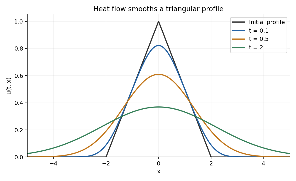
The profile is an even function, so its Fourier transform is real andFor $\omega \ne 0$, integration by parts givesThereforeAt zero, direct integration gives the area of the triangle, namely two; the displayed quotient has the same limit. In particular $\hat{T}(\omega )\ge 0$ for every real frequency. This is the Fourier transform of a triangular function.

One can also see the nonnegative square structurally: $T=\frac{1}{2}{1}_{[-1,1]}\ast 1_{[-1,1]}$, so the convolution theorem gives $\hat{T}=\frac{1}{2}(2\sin \omega /\omega {)}^2$.

Complete the square inside the Fourier transform of the Gaussian heat kernel:After $z=x/(2\sqrt{t})$,The supplied shifted Gaussian integral equals $\sqrt{\pi }$ for real $\sqrt{t}\omega$. HenceAt zero this says $\int q_t=1$, so convolution with the heat kernel averages rather than rescales the initial mass. The formula is an instance of the Fourier transform of a Gaussian.

Both kernels are integrable functions, so the convolution theorem givesThe uniqueness of the Fourier transform on integrable functions gives equality almost everywhere. Both sides are continuous, so it holds at every point:For completeness, continuity of the convolution follows by dominated convergence: $q_t$ is bounded and continuous, so for $x_j\to x$ the integrands $q_t(x_j-y)q_s(y)$ converge pointwise and are dominated by $\Vert q_t{\Vert }_{\infty }{q}_s(y)$.

The identity is the heat semigroup property: evolving for time $s$, then for time $t$, is the same as evolving once for time $s+t$.

For fixed frequency $\omega$, the Fourier transform of a derivative gives $\widehat{u_{xx}}=-{\omega }^2\hat{u}$. The transformed initial value problem is thereforeSolving this scalar ordinary differential equation yieldswhere the value at $\omega =0$ is interpreted by continuity and equals two. Thus diffusion suppresses high frequencies by the Gaussian multiplier while preserving the zero-frequency mass.

The differentiation and transform steps are justified for the heat kernel solution $u=q_t\ast T$: for positive time its spatial derivatives are integrable, since Gaussian derivatives are integrable and $T$ is bounded with compact support. Alternatively, the transformed calculation first suggests the formula, and the next part verifies the resulting solution directly.

Insert part (i) in the inverse Fourier transform. The factor two in $\hat{T}$ cancels half of the inverse normalization:The integrand has a removable singularity at zero. For $t>0$, the Gaussian controls every polynomial factor at infinity, so differentiation under the integral is valid. Differentiation in $t$ and twice in $x$ both multiply the integrand by $-{\omega }^2$, proving $u_t=u_{xx}$.

There is also a direct physical-space representation:Since $q_t$ has integral one, writeThe continuous compactly supported profile $T$ is uniformly continuous. Given $ϵ>0$, choose $\delta >0$ so its change is below $ϵ$ for $|y|<\delta$. That part of the integral is bounded by $ϵ$. The other part is bounded by $2\Vert T{\Vert }_{\infty }{\int }_{|y|\ge \delta }{q}_t(y)dy$, which tends to zero by the substitution $y=2\sqrt{t}z$ and the vanishing tails of the Gaussian integral. This proves $u(t,x)\to T(x)$ uniformly as $t\downarrow 0$ and verifies the initial condition.

Thus the formula supplies the full heat evolution of a triangular profile, including the corner points of the initial profile. Positive time immediately smooths those corners.