Past exam of the approximation theory and finite element methods course of the University of Oxford / 2009 / A (Approximation Theory)

Define the Lagrange cardinal polynomialsDistinct nodes make every denominator nonzero. At $x_s$ these polynomials satisfy ${\ell }_r(x_s)={\delta }_{rs}$, so the Lagrange interpolation polynomial isIt has degree at most $n$ and takes the prescribed data values. If two such polynomials existed, their difference would have $n+1$ distinct roots but degree at most $n$, forcing that difference to be zero. This also proves uniqueness.

With $w_s=1/{\pi }_{n,s}(x_s)$, the Lagrange interpolation polynomial can be written, away from its nodes,Apply the same formula to the constant data $u_s=1$. Uniqueness of polynomial interpolation gives ${\sum }_s{\ell }_s=1$, and henceDivide the two identities to obtain the barycentric interpolation formulaAt $x=x_r$, use the continuous limiting value $u_r$. Multiplying every weight by the same nonzero constant cancels between numerator and denominator, so only relative weights are needed in computation.

For uniformly spaced nodes,There are $n-s$ negative factors, coming from $j>s$. Thus the weights fixed by part (b) satisfy this formula exactly. The printed sign $(-1{)}^s$ agrees for even $n$; for odd $n$ it differs by the common factor $-1$. Rescaling all weights by $(-1{)}^n$ gives the printed convention without changing the barycentric interpolation formula.

For even $n$, the required magnitude isStirling's formula givesThus central weights are exponentially larger in magnitude than endpoint weights. Their alternating signs can cause severe cancellation in polynomial interpolation at equispaced nodes; they reflect the unfavorable high-degree interpolation geometry associated with Runge's phenomenon. A barycentric evaluation formula improves the implementation but does not remove the intrinsic sensitivity or guarantee convergence for every smooth function. The comparison with the bounded relative weights at Chebyshev-Lobatto nodes is decisive.

Use the Chebyshev polynomial identities $T_0=1$, $T_1=x$, and $T_{j+1}=2x{T}_j-T_{j-1}$. Induction shows that $T_j$ has degree $j$ with leading coefficient $2^{j-1}$ for $j\ge 1$. The trigonometric definition also givesThereforeThe leading coefficient is $2^{1-n}{n}^{-1}\cdot n{2}^{n-1}=1$, and the degree is $n+1$. The endpoints are roots through $x^2-1$; the other $n-1$ points $\cos (s\pi /n)$ are roots through $T_n^{\prime }$. They are distinct, so this monic polynomial is exactly ${\pi }_n$.

Differentiating the product ${\pi }_n(x)=(x-x_s){\pi }_{n,s}(x)$ at $x_s$ gives ${\pi }_n^{\prime }(x_s)={\pi }_{n,s}(x_s)=w_s^{-1}$. For an interior node, differentiate the trigonometric form using $d/dx=-(\sin \theta {)}^{-1}d/d\theta$:At ${\theta }_s=s\pi /n$, this is $2^{1-n}n(-1{)}^s$. At either endpoint, taking the limit makes the two terms equal, doubling the value: ${\pi }_n^{\prime }(x_s)=2^{2-n}n(-1{)}^s$ for $s=0,n$.

After removing the common factor $2^{n-1}/n$, the barycentric interpolation formula therefore usesThese Chebyshev-Lobatto node weights differ in magnitude by only a factor of two.

Let $t_1,\dots ,t_m$ be the distinct roots in $(0,1)$ at which ${\varphi }_r$ changes sign, and put $q(x)={\prod }_{j=1}^m(x-t_j)$. Both ${\varphi }_r$ and $q$ change sign at each such point, while roots of even multiplicity do not change sign. Consequently ${\varphi }_{r}q$ has one constant sign on $(0,1)$ except at its zeros, and is not identically zero. Its integral cannot vanish.

If $m<r$, however, orthogonality of the monic orthogonal polynomial ${\varphi }_r$ to every polynomial of lower degree gives $({\varphi }_r,q)=0$, a contradiction. Hence $m\ge r$. Since $\mathrm{deg}{\varphi }_r=r$, there must be exactly $r$ such roots, each of multiplicity one. They exhaust the degree, leaving no complex, exterior, or endpoint roots. Thus all roots are simple and lie strictly in $(0,1)$, which proves the requested weaker inclusion in $[0,1]$. This is the sign-change proof of the zeros of orthogonal polynomials theorem.

The monic orthogonal polynomials ${\varphi }_0,\dots ,{\varphi }_{r+1}$ form a basis of $P_{r+1}$, ordered by degree. Since $x{\varphi }_r$ is monic of degree $r+1$,For $j\le r-2$, symmetry of multiplication by $x$ gives $(x{\varphi }_r,{\varphi }_j)=({\varphi }_r,x{\varphi }_j)=0$, because $\mathrm{deg}(x{\varphi }_j)<r$. Only $a_r$ and $a_{r-1}$ remain. Taking inner products with ${\varphi }_r$ yields $a_r=({\varphi }_r,x{\varphi }_r)/({\varphi }_r,{\varphi }_r)$.

Similarly,since $x{\varphi }_{r-1}-{\varphi }_r$ has degree at most $r-1$. Rearranging proves the three-term recurrence for monic orthogonal polynomials:

The monic degree-zero polynomial is ${\varphi }_0=1$. Orthogonality of $x-a$ to one gives $a={\int }_0^{1}xdx=1/2$, so ${\varphi }_1=x-1/2$.

The relevant integrals areInsert these into the three-term recurrence for monic orthogonal polynomials:ThusTheir mutual orthogonality can also be checked directly by integrating on $[0,1]$.

The best approximation in the $L^2$ norm is the orthogonal projection onto $\mathrm{span}\{{\varphi }_0,{\varphi }_1\}$. ThereforeUsing ${\int }_0^1{x}^{k}dx=1/(k+1)$,It follows thatThe error is orthogonal to every linear polynomial, so the Pythagorean identity proves optimality and uniqueness. At $k=0$, this gives $p_1=1$; at $k=1$, it gives $p_1=x$. Both are exact because the target itself then belongs to $P_1$.

Put $x=1-t$. For $0<k\le 1$,whereas the constrained rational interpolant expands asMatching the constant term gives $a=1+b$, and matching the coefficient of $t$ gives $1/(1+b)=k$. Thus $a=1/k$, $b=(1-k)/k$, andThis is an endpoint-constrained rational approximation to a power: it matches value and derivative at $x=1$ and also enforces $r(0)=0$ for $k>0$.

There is a terminology qualification. A standard degree-$(1,1)$ Padé approximant about $t=0$ matches through $t^2$, but the displayed constrained expression has quadratic coefficient $-k(1-k)$ rather than $-k(1-k)/2$. The unconstrained Padé approximant is insteadThe source's requested formula is obtained by the two stated endpoint matching conditions within its restricted family, rather than by full Padé matching. At $k=1$ both reduce to $x$. At $k=0$, the requested expression is one for $x>0$ with a removable value at zero; finite $a,b$ in the original restricted form do not represent that constant function. The endpoint is understood by this limit.

By definition, a best uniform approximation $p^{\ast }\in P_n$ minimizes $\Vert u-p{\Vert }_{\infty }$ over $p\in P_n$. Write $E=\Vert u-p^{\ast }{\Vert }_{\infty }$. The equioscillation theorem says that, if $E>0$, optimality is equivalent to the existence of $n+2$ ordered points with signed errorsThe absolute-value bars on the left of the printed formula must be omitted for this alternating-sign statement. A nonnegative absolute value cannot equal a negative $-E$.

For sufficiency, suppose a polynomial $p$ had strictly smaller error. At the alternating points, $p-p^{\ast }$ must have the same sign as $u-p^{\ast }$, since otherwise the new error would have magnitude at least $E$. The difference polynomial therefore changes sign in all $n+1$ successive gaps and has at least $n+1$ distinct roots, impossible for a nonzero element of $P_n$.

For necessity, suppose that no $n+2$ alternating extremal points exist. On the compact extremal set $K=\{x:|u(x)-p^{\ast }(x)|=E\}$, group the signs of the error into consecutive blocks. The positive and negative extremal sets are disjoint compact sets, so sign changes are separated by positive distances; the number of blocks is finite. The absence of an $n+2$ alternating selection means there are at most $n+1$ blocks. Place a root in each gap between successive blocks and choose the overall sign of their product $q$ to agree with the error on $K$. Then $\mathrm{deg}q\le n$ and $q$ is nonzero throughout $K$.

By compactness and continuity, on a neighborhood of $K$ the signs still agree and $|q|$ is bounded below. A sufficiently small positive $\eta$ reduces the error there when $p^{\ast }$ is replaced by $p^{\ast }+\eta q$. On the compact complement of this neighborhood the old error is below $E$ by a fixed positive margin, and choosing $\eta$ smaller preserves that margin. This gives a strictly better approximation, a contradiction. If $E=0$, the target already lies in $P_n$ and optimality is immediate.

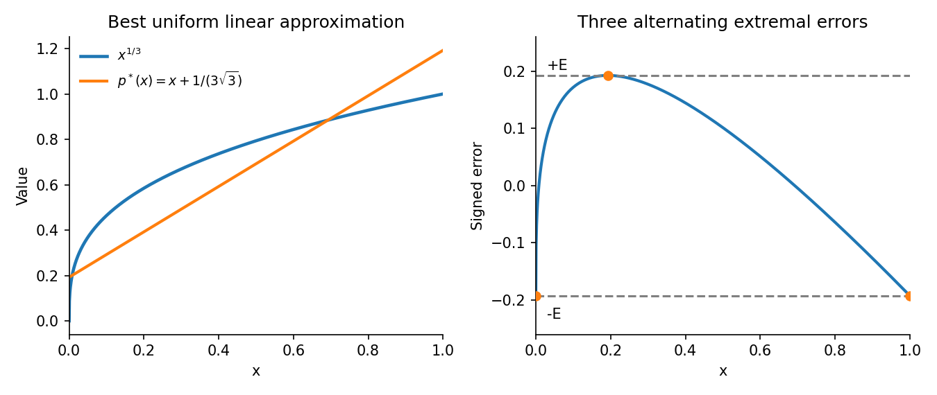
For $u(x)=x^{1/3}$, the chord is $x$. Concavity gives $x^{1/3}-x\ge 0$, with maximum at $x_{\ast }=1/(3\sqrt{3})$ and maximum value $2/(3\sqrt{3})$. Shift the chord up by half that amount. The errors at $0,x_{\ast },1$ are respectively $-E,+E,-E$, so

Use the standard meaning of a cubic spline: a $C^2$ function that is cubic on each unit interval. If it vanishes on both exterior intervals, continuity of the function and its first two derivatives gives zero endpoint jets at zero and at $k$.

Such a spline can be represented through its third-derivative jumps asFor $x\ge k$, this must be the zero polynomial. Expanding in powers of $x$ yields the four moment conditionsIf $k\le 3$, the columns of this Vandermonde system are linearly independent, so every $c_j=0$. No nonzero spline has such short support.

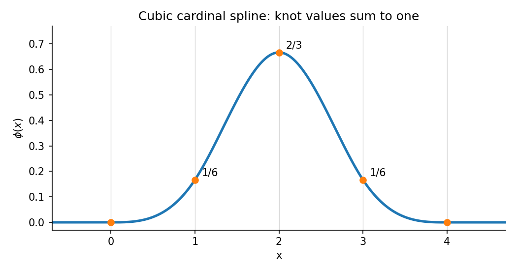
For $k=4$, a nonzero null vector is $(1,-4,6,-4,1)$, since the fourth finite difference annihilates every cubic. Thus the Cardinal cubic B-spline isIts knot values at $0,1,2,3,4$ are $0,1/6,2/3,1/6,0$, whose sum is one. It is nonzero and supported on $[0,4]$, proving the minimal value $k=4$. Equivalently, on $[0,1]$ it is $x^3/6$, on $[1,2]$ it is $[-3x^3+12x^2-12x+4]/6$, and the other half follows by symmetry $\varphi (4-x)=\varphi (x)$.