TODO — user-deferred biology. This biological subquestion is intentionally left unsolved under the current scope.
TODO — user-deferred biology. This biological subquestion is intentionally left unsolved under the current scope.
TODO — user-deferred biology. This biological subquestion is intentionally left unsolved under the current scope.
TODO — user-deferred biology. This biological subquestion is intentionally left unsolved under the current scope.
TODO — user-deferred biology. This biological subquestion is intentionally left unsolved under the current scope.
TODO — user-deferred biology. This biological subquestion is intentionally left unsolved under the current scope.
TODO — user-deferred biology. This biological subquestion is intentionally left unsolved under the current scope.
Use symmetric single-bead displacements with the Metropolis acceptance rule, discard equilibration, and record the end-to-end distance after complete sweeps, including sweeps with rejected moves. One sweep is attempted bead moves; it is a sampling index, not physical time.
INITIALIZE(N, sigma):
    for i = 1,...,N:
        r[i] = ((i-1)*sigma, 0, 0)
    return r

ENERGY(r):
    for each pair i < j:
        if norm(r[i]-r[j]) < sigma:
            return infinity
    U = 0
    for i = 1,...,N-1:
        U += k/2 * (norm(r[i+1]-r[i])-sigma)^2
    return U

TRIAL(r):
    choose i uniformly from 1,...,N
    choose delta uniformly from [-a,a]^3
    r_trial = copy(r)
    r_trial[i] += delta
    return r_trial

ACCEPT(U, U_trial, beta):
    if U_trial == infinity:
        return false
    return log(uniform(0,1)) < min(0, -beta*(U_trial-U))

MAIN:
    r = INITIALIZE(N, sigma)
    U = ENERGY(r)
    for sweep = 1,...,n_equilibrate+n_produce:
        repeat N times:
            r_trial = TRIAL(r)
            U_trial = ENERGY(r_trial)
            if ACCEPT(U, U_trial, 1/(k_B*T)):
                r = r_trial
                U = U_trial
        if sweep > n_equilibrate:
            d_ETE = norm(r[N]-r[1])
            store d_ETE and update its histogram
    estimate autocorrelation and block uncertainties
The straight initial chain is nonoverlapping and has zero bond-stretching energy, but is not presumed to be an equilibrium configuration. Check relaxation from contrasting initial configurations and stationarity before production. The displacement scale may be tuned during equilibration and then held fixed. Every sweep may be recorded; correlations are handled in uncertainty estimates rather than pretending adjacent records are independent. If thinning is used, choose its spacing with reference to the measured autocorrelation time. Rejected states must still be sampled to retain their correct equilibrium residence weight.
For a chosen bead, the uniform displacement cube is inversion symmetric, so the proposal distribution satisfies . The target canonical density is for allowed configurations. With ,This proves detailed balance. Overlapping trials have zero target weight and are rejected. The proposal must retain rejected trials as self-transitions; repeatedly proposing until a nonoverlapping move appears would generally introduce a configuration-dependent proposal normalization and need a Hastings correction. Detailed balance establishes stationarity, while sufficient sampling also requires practical exploration of the accessible state space.
The hard-core chain does not undergo an energetic low-temperature collapse. For allowed configurations the only finite energy is bond stretching. If , bond lengths remain near and temperature mostly changes the small bond-length fluctuations, not the distribution of angular conformations. The end-to-end distance therefore fluctuates over an expanded self-avoiding-coil distribution even at low temperature, with an approximate scale and for sufficiently long three-dimensional chains.
For , the scaling is qualitative and finite-chain effects matter. An equilibrated distance-versus-sweep trace is stationary, with correlated excursions; a histogram of that trace is a distinct plot, not a curve of probability density against simulation step. Neither the temperature in kelvin nor the spring constant is specified, so an exact histogram cannot be calculated. The illustrative figure compares like-for-like coil traces rather than asserting a unique numerical simulation result.
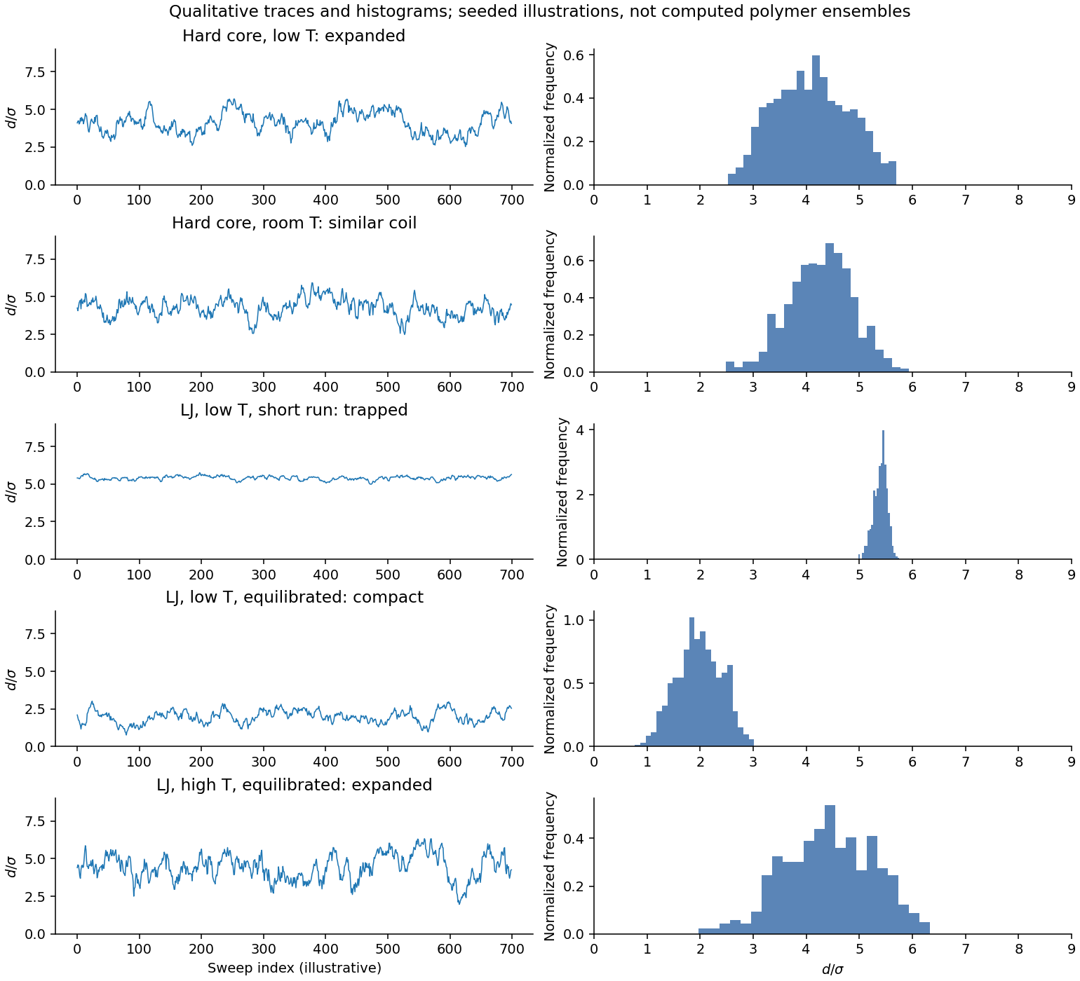
Original qualitative Monte Carlo traces and end-to-end-distance distributions for repulsive and attractive chains
. Details. 
At room temperature, the same hard-core exclusion remains temperature independent. If the spring remains stiff, the conformational distribution remains broadly similar to the low-temperature expanded-coil distribution. Finite bond-length fluctuations increase with and can slightly enlarge the length scale and distribution width. The radial bond measure also favours lengths slightly above the harmonic minimum.
The comparison depends on the dimensionless stiffness , not on the word “room” alone. There is no attractive energy in this model to produce a low-temperature globule and high-temperature coil transition. Monte Carlo decorrelation speed can change with temperature and proposal scale, but the premise already stipulates adequate equilibrium sampling in both cases.
With an attractive Lennard-Jones potential and , a short run can remain trapped in an initial conformation or a metastable compact state. A distance trace may show a long apparently stationary segment, an initial collapse, or occasional jumps between local structures; its histogram depends on initialization and is not necessarily an equilibrium distribution. An extended start need not collapse on the available run length, and a compact start need not already be the global minimum.
Accepting only downhill moves would make this trapping worse and would not sample the specified finite-temperature canonical ensemble. The sketch should therefore label this trace as unequilibrated and avoid assigning its mean a thermodynamic interpretation.
For a genuinely equilibrated low-temperature attractive chain, many nonbonded contacts lower the energy. Compact conformations normally dominate, giving a smaller characteristic end-to-end distance than the high-temperature coil. The trace can remain near particular compact basins for long periods but must, under the stated premise, sample their correct equilibrium weights. The end-to-end distribution may have structure associated with distinct compact shapes; the end beads need not be nearest neighbours, so a compact globule does not force .
For there is a rounded finite-system crossover rather than a sharply defined bulk coil–globule phase transition. The exact histogram requires the dimensionless temperature, stiffness and treatment of bonded-pair Lennard-Jones interactions, none of which is numerically specified.
At , attractive contact energies are weak compared with thermal fluctuations, so expanded coil-like conformations are favoured and the end-to-end distribution broadens towards larger distances. Strong short-range repulsion still limits overlap over an effective, temperature-dependent diameter. The soft Lennard-Jones model is therefore not exactly identical to a temperature-independent hard-sphere chain, even when attraction is relatively unimportant.
A sufficiently stiff spring keeps the chain contour length near in all three comparisons. If temperature instead becomes comparable with , increased bond stretching introduces an additional size change and the intended fixed-bond coil comparison breaks down. Every equilibrated trace should fluctuate around a stationary distribution; an expanding running mean caused by incomplete relaxation is not evidence for an equilibrium high-temperature state.
Articles by others on the same topic
There are currently no matching articles.