Past exam of the computer science course of the University of Oxford / 2018 / Algorithms (A16156W1)

Solutions to all three questions of the University of Oxford computer science finals paper, Trinity Term 2018, held on 16 June 2018. Every printed option is treated.

Source: Public examination-paper archive, member 2017/T/a16156w1.pdf, paper A16156W1, three scanned pages. The printed 2018 cover controls the sitting despite the archive member’s directory name.

A binary search tree is a binary tree storing distinct keys from a total order, with every key in a node's left subtree smaller than that node's key and every key in its right subtree larger. The condition concerns entire subtrees, not just immediate neighbours.

For membership, start at the root of a tree and compare the target with the current key. Return true on equality; continue into the left subtree for a smaller target and the right subtree for a larger target; return false on an empty subtree. The binary search tree ordering ensures that a discarded subtree cannot contain the target. Each step descends one level, so the algorithm terminates and uses $O(h+1)$ time complexity for height of a binary tree $h$, under constant-time key comparison.

First perform splaying on the key to be deleted, making its node the root of a tree. Delete that root, leaving left and right subtrees $L,R$. If either is empty, return the other. Otherwise find the maximum key $m$ of $L$ by following right-child references, and perform splaying on $m$ within $L$. This makes $m$ the root of $L$ with an empty right subtree. Attach $R$ there. The result is the original splay tree with exactly the selected key removed. An unsuccessful lookup leaves the represented set unchanged.

For algorithm correctness, all keys of $L$ are smaller than the deleted key, and all keys of $R$ are larger. Splaying preserves the binary search tree property by the permitted assumption. Since $m$ is the maximum of $L$, it has no larger key within $L$; since every key of $R$ exceeds $m$, attaching $R$ as its right subtree preserves every ordering condition. All remaining keys occur once. This is the join-based deletion of a splay tree.^[ref]

No. In a red-black tree with no red nodes, equal black height forces every graph path from the root to an absent-child position to have the same length. A real node cannot have exactly one real child: the two paths through that node would then have different numbers of black nodes. Recursively, every real level must be full. The tree is therefore a perfect binary tree.

With $h$ real levels its size is $1+2+\cdots +2^{h-1}=2^h-1$. A size of $23$ would require $2^h=24$, which is impossible for an integer $h$. The black null sentinels are not counted among the $23$ stored entries. This is the all-black red-black tree size criterion.

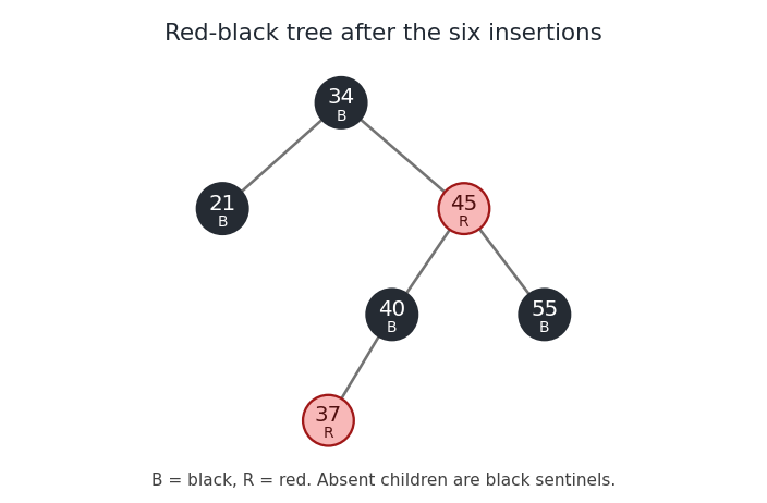
Use the conventional bottom-up red-black tree insertion: insert a red node by the binary search tree rule, repair a red parent with recolouring or tree rotations, and make the root black. Write $B$ and $R$ for black and red. The first three insertions give root $34_B$, with $21_R$ on the left and $55_R$ on the right.

Inserting $40$ as the left child of $55$ gives a red parent and a red uncle. Recolour $21,55$ black and retain a black root $34$. Inserting $45$ then gives the inner configuration $55_B$–$40_R$–$45_R$. A left tree rotation at $40$, followed by a right tree rotation at $55$, produces a subtree rooted at $45_B$ with $40_R$ and $55_R$ beneath it. Finally insert $37_R$ to the left of $40_R$. Its uncle $55_R$ is red, so recolour $40,55$ black and $45$ red. No further repair is required because $45$ has black parent $34$.

The final root is $34_B$; its left child is $21_B$ and its right child is $45_R$. Under $45_R$ are $40_B$ on the left and $55_B$ on the right; $40_B$ has left child $37_R$. All omitted children are black null sentinels. Each root-to-null graph path has two real black nodes, and no red node has a red child.

Write $y=x+1$. After splaying on $x$, that key is at the root, and $y$ is the smallest key in its right subtree. This uses the integer assumption: no stored key lies strictly between $x$ and $y$. Thus $y$ has an empty left subtree while it remains within the right subtree of $x$.

Now perform ordinary bottom-up splaying on $y$. Until the final step involving $x$, all tree rotations occur below $x$ and leave it at the root. There are only two possible final cases.

Therefore $x$ becomes the left child of $x+1$. The argument applies more generally to consecutive keys in a binary search tree, even when their numerical difference is not one.

Use the usual bottom-up splaying operations. We prove the stronger result that at most three successful calls suffice. No insertions or deletions are needed.

If the chosen key $x$ is the minimum stored key, first perform splaying on $x$ and then on its immediate successor. The argument for consecutive keys in a binary search tree makes $x$ the left child of the successor with an empty right subtree; minimality makes its left subtree empty too. Hence $x$ is a leaf of a rooted tree. The maximum-key case is the mirror image.

Suppose $x$ is an interior key. Since at least four keys are stored, there are either two keys larger than $x$ or two smaller than $x$. In the former case choose four consecutive stored keyswhere $a$ is the predecessor of $x$, and $b,c$ are the next two successors. Perform $\mathrm{Splay}(c),\mathrm{Splay}(a),\mathrm{Splay}(b)$.

Here is a complete check of the local shapes. After the first call, $c$ is the root. After the second, $a$ is the root; every key below $a$ is in its left subtree $A$, and every key above $c$ stays in the right subtree $D$ of $c$. These outside subtrees cannot interfere with the next search. Between $a$ and $c$ there are only $x,b$. The last step of splaying on $a$ is either a zig step, leaving $c$ as its right child; a zig-zag step, with the same result; or a zig-zig step, leaving some $p\in \{x,b\}$ as its right child with $c$ immediately to the right of $p$. Consequently the possible right subtrees of $a$ are exactly among these four forms, using $k(L,R)$ for a node with its left and right subtrees:Here an unexpanded $x$ or $b$ denotes a node with no children. Each row follows by the indicated one or two tree rotations in each bottom-up step. All rows end with $x$ as the right child of $a$, with both its subtrees empty. If instead two keys below $x$ are available, reflect the construction, exchanging left and right and reversing the order of keys. This proves splaying a chosen node into a leaf for every node of every splay tree of size at least four.

For a finite undirected graph $G=(V,E)$, a vertex cover is a subset $C\subseteq V$ meeting every edge: for every $\{u,v\}\in E$, at least one of $u,v$ belongs to $C$. The optimization problem asks for a vertex cover of minimum cardinality. Its usual decision version also supplies an integer $k$ and asks whether one exists with $|C|\le k$.

Construct a set cover problem instance whose universe is the set of edges $E$. For each vertex $v\in V$, supply the set $S_v$ of all edges incident to $v$. A collection $\{S_v:v\in C\}$ covers the universe if and only if every edge has an endpoint in $C$, which is precisely the vertex cover condition.

The correspondence preserves cardinality: a vertex cover of size $k$ is a feasible solution of the set cover problem using $k$ of these sets, and conversely. If two labelled vertices produce identical sets, one can keep their labels or discard duplicate choices without changing the optimum. The construction has size $O(|V|+|E|)$ when incidences are listed, so it is a polynomial-time reduction.

Root the tree arbitrarily. For each vertex $v$, let $D_1(v)$ be the minimum vertex cover size in its descendant subtree, conditional on selecting $v$, and $D_0(v)$ the corresponding minimum conditional on omitting $v$. Process the vertices in postorder traversal. For every child $u$ of $v$,At a leaf of a rooted tree, the empty sums give $D_1=1,D_0=0$. Return $\min \{D_0(r),D_1(r)\}$ at the root $r$.

For algorithm correctness, if $v$ is selected, each child subtree may independently use its cheaper state, since the connecting edge is already covered by $v$. If $v$ is omitted, each child must be selected to cover its connecting edge. Distinct child subtrees have no edges between them because the input is a tree. These observations prove the recurrences by structural induction. Each edge contributes constant work once, giving $O(|V|)$ time complexity and $O(|V|)$ space with adjacency lists. The single-vertex tree correctly has optimum zero. This is minimum vertex cover of a tree by dynamic programming.

In depth-first search of an undirected graph, every edge joins a vertex to one of its ancestors or descendants in the discovery tree. To see this directly, suppose $u$ is discovered before its neighbour $v$. If $v$ is still undiscovered, the search from $u$ cannot finish before discovering $v$: it eventually scans $uv$. Thus $v$ is discovered while the call for $u$ remains active and belongs to its descendant subtree.^[ref]

For any edge $uv$, its ancestor endpoint therefore has a proper descendant and hence at least one child. It is an internal vertex of a rooted tree. Every edge has an internal endpoint, so the internal vertices form a vertex cover. The relevant leaves of a rooted tree here have no children in the rooted discovery tree; a root of vertex degree one can still be internal.

We construct an injection from the unmatched vertices in a matching to the leaves of a rooted tree. Start a downward graph path at each unmatched vertex $u$. If the current vertex is a leaf of a rooted tree, stop. Otherwise choose any child $v$. The current vertex is either the unmatched starting point or a vertex already matched to its own parent.

In either case, $v$ cannot be unmatched: the proper matching in a rooted tree condition would require its parent to be matched to one of $v$'s siblings in a rooted tree, whereas that parent is either unmatched or already matched upward. Nor can $v$ be matched to its parent. Its matching partner must therefore be one of its own children, say $w$. Extend the graph path by the two edges to $v$ and then to $w$, and continue from $w$.

Every extension descends two levels, so finiteness guarantees termination at a leaf of a rooted tree. Every visited vertex except the starting point is matched. The constructed graph paths for different unmatched starting points are disjoint: if two downward graph paths in a tree meet, one starting point must lie on the other path, which would put a second unmatched vertex after the first. That is impossible. Hence their terminal leaves of a rooted tree are distinct, provingOnly the properness condition for unmatched non-root vertices was used. If the root is unmatched and the convention exempts it because it has no parent, the same construction starts there and still works. Thus the root convention does not affect the claimed inequality. This proves the unmatched-vertex bound for a proper tree matching without requiring $M$ to have maximum size.

For a connected graph with at least one edge, run depth-first search and output the set $I$ of internal vertices of a rooted tree in its discovery tree $T$. Part (d) proves that $I$ is a vertex cover. It is also connected: every ancestor of an internal vertex is internal, so the graph path in $T$ from that vertex to the root stays inside $I$. The root is internal when $|V|\ge 2$.

For the approximation guarantee, choose a maximum-size proper matching in a rooted tree $M$ of $T$, whose existence is supplied. It is used only in the analysis; the algorithm need not construct it. Since every matched edge uses two distinct vertices,By part (e), $|L(T)|\ge |U(M)|$. ThereforeThe final inequality holds because every vertex cover of $G$, connected or otherwise, must use at least one distinct endpoint for each of the disjoint edges in $M\subseteq E(G)$. Thus this is a 2-approximation algorithm in $O(|V|+|E|)$ time complexity.

For completeness, a disconnected input needs a feasibility check: if two different connected components of a graph contain edges, no connected vertex cover can meet both. If exactly one component contains edges, run the construction on that component and ignore isolated vertices. If there are no edges, the empty vertex cover is optimal when an empty solution is permitted; if a nonempty connected solution is required, any single vertex is optimal for a nonempty input. These conventions cover the boundary cases omitted from the main approximation argument.

Use the standard maximum form of a linear programAn arbitrary linear program can be converted by the following operations.

These substitutions preserve the attainable objective values, up to the stated sign and constant corrections, and map feasible points in both directions. An alternative standard-form convention uses $Az=b,z\ge 0$: add a nonnegative slack variable to each upper-bound row, or subtract a nonnegative surplus variable from a lower-bound row. The inequality convention above is used in the remaining solutions.

Let $Z$ be the set of isolated vertices of the finite simple graph $G=(V,E)$. Introduce a nonnegative integer $x_v$ for every vertex. Use the integer programEvery nonisolated vertex belongs to an edge, whose inequality and the other endpoint's nonnegativity already imply $x_v\le 1$. The explicit bounds on $Z$ therefore make all variables binary. For an integer feasible point, $S=\{v:x_v=1\}$ is an independent set, and its cardinality is the objective. Conversely the indicator vector of any independent set is feasible. Thus the optimal value is the maximum independent set size. Including the isolated-vertex bounds is essential for an arbitrary graph; without them the formulation would be unbounded whenever an isolated vertex is present.

Remove the integer requirements from the previous formulation to obtain its linear programming relaxation. Give each edge constraint a nonnegative dual variable $y_e$, and each bound for $v\in Z$ a nonnegative dual variable $z_v$. Since all right-hand sides are one, the dual linear program isAn integer feasible point selects a multiset of edges touching every nonisolated vertex, together with at least one singleton for each isolated vertex. Repeated edges or singleton choices can be discarded without losing coverage, so an optimum has a genuine edge cover of the nonisolated part and one singleton per isolated vertex. If $G$ has no isolated vertices, this is exactly an edge cover, with the objective counting selected edges including any unnecessary multiplicities. The isolated-singleton extension is necessary because a graph with an isolated vertex admits no ordinary edge cover.

This interpretation concerns integer feasible dual solutions. The linear programming relaxation can have fractional optima, so its value need not equal the integer independent set optimum. For example, the triangle has relaxed independent-set value $3/2$, whereas its maximum independent set has size $1$ and its minimum edge cover has size $2$.

Regard the two kinds of agents as the two sides of a complete bipartite graph, with edge weight $c_{ij}$. Pairing everyone is a perfect matching, and its maximum total weight is $P$. Consider the capacitated linear programIt is feasible and bounded. Every optimum has all row and column sums equal to one: otherwise the equal total deficits of the two sides give a row $i$ and column $j$ both below one. Increasing $x_{ij}$ by the smaller of their positive deficits remains feasible and increases the objective because $c_{ij}>0$, a contradiction.

Thus an optimum is a doubly stochastic matrix. By the Birkhoff-von Neumann theorem it is a convex combination of permutation matrices, so at least one corresponding perfect matching has weight at least its objective. Conversely every such perfect matching gives a feasible matrix. Hence $P_{\mathrm{LP}}=P$. One way to justify the decomposition is to apply Hall's marriage theorem to the positive-entry support, subtract the smallest entry on a supported perfect matching, and repeat after rescaling the nonzero remainder; each subtraction removes a positive entry, so the process terminates.

The dual linear program assigns nonnegative dual variables $p_i,q_j$ to the row and column capacity constraints:These are exactly the permitted payments and all the pairwise acceptance conditions, so its optimal value is $Q$. It is feasible, for example by taking $p_i={\max }_j{c}_{ij}$ and $q_j=0$. Strong duality now gives $P=P_{\mathrm{LP}}=Q$. In particular, the nonnegative payment restriction has been retained throughout; using capacity inequalities rather than equality constraints avoids introducing unrestricted prices.

For a direct weak duality check, sum $p_i+q_{\pi (i)}\ge c_{i,\pi (i)}$ over any pairing $\pi$. Its revenue never exceeds the company's total offered payment. The linear programming duality and integrality argument prove that this lower bound on payments is attained.

Combine all inequalities, including nonnegativity, into $Cx\le d$; explicitly, the rows $-e_j^{T}x\le 0$ encode $x_j\ge 0$. Let $x_{\ast }$ be a vertex of a linear polyhedron, equivalently an extreme point of the feasible linear polyhedron, and let $I$ index the active constraints there.

Suppose the active row normals have rank smaller than $n$. By the rank-nullity theorem there is a nonzero vector $h$ with $C_{i}h=0$ for every $i\in I$. Every inactive row has positive slack variable value $s_i=d_i-C_i{x}_{\ast }>0$. Since there are only finitely many rows, choose $\epsilon >0$ so small thatThen both $x_{\ast }+\epsilon h$ and $x_{\ast }-\epsilon h$ are feasible points: the active constraints remain equalities and no inactive inequality is violated. They are distinct, and $x_{\ast }$ is their midpoint, contradicting the extreme point property.

Therefore the active row normals have rank $n$, and at least $n$ linearly independent constraints are satisfied with equality. In particular at least $n$ constraints are tight, as claimed. Nonnegativity bounds must be counted: for example, at the origin these can supply all $n$ active rows. Degeneracy can make more than $n$ constraints tight, so the result does not assert exactly $n$.