Past exam of the computer science course of the University of Oxford / 2019 / Artificial intelligence (A16607W1)

Source paper: released Oxford examination archive, member 2018/T/a16607w1.pdf. Its native cover identifies the Second Public Examination, Trinity Term 2019, Monday 3 June, 14:30–16:30. The archive directory predates the actual cover year. All three questions and every unnumbered requirement within their printed parts are addressed. The blocks-world figure is intact.

The first assertion is false. Give the root a first child that is a goal state of cost ten and another child leading to many cheaper non-goal search nodes. Depth-first search can take the first child and stop immediately. A-star search with the admissible heuristic $h=0$ behaves as uniform-cost search and expands the cheaper non-goal search nodes before selecting that goal. Thus an admissible heuristic does not make A-star search expand fewer nodes than every possible depth-first search ordering. The latter need not return an optimal solution.

The second assertion is true under the usual finite-branching factor assumption. Breadth-first search orders by search depth, not path cost. Every finite depth contains finitely many search nodes, so a goal at finite depth is eventually reached even if some steps cost zero. Zero-cost steps can affect cost optimality, but do not obstruct this completeness argument. An infinite branching factor would invalidate the argument irrespective of step costs.

The third assertion is true as a worst-case black-box requirement, with a finite optimum assumed. If outgoing actions are known only by expanding a state, an unexamined reachable branch can conceal a sufficiently negative-cost action followed by a route to a goal. Its total cost can beat the current solution by an arbitrarily large amount. Without additional lower bounds or structural information, finding one cheap solution cannot justify stopping; exhaustive examination can be necessary. This does not assert that every already-described irrelevant state must be visited on every input. Moreover, a reachable negative-cost cycle in a graph that can still reach a goal can make costs unbounded below, in which case no finite-cost optimal solution exists at all.

Iterative deepening depth-first search increases a bound on the number of actions, usually through $0,1,2,\dots$. Iterative lengthening search instead bounds accumulated path cost; after an unsuccessful pass, its next bound is the least path cost among the rejected search nodes. Thus it can distinguish shallow expensive paths from deeper cheap ones.

Both repeatedly perform depth-first search and retain its small active-path storage, trading repeated work for avoiding a large search frontier. With unit step costs their bounds coincide. With unequal positive step costs, iterative deepening depth-first search finds a solution with the fewest actions, while iterative lengthening search, under the termination conditions discussed next, finds one of least total cost. Real-valued path costs can make iterative lengthening search perform many more passes than the depth-bounded method.

Start the threshold at zero and let $C^{\ast }$ be the least solution cost. Suppose an unsuccessful pass has threshold $L<C^{\ast }$. Along an optimal action sequence, take the first prefix whose path cost exceeds $L$. Its preceding prefix is explored, so that rejected prefix contributes to the next-threshold calculation. Positive step costs imply that its cost is at most $C^{\ast }$. Therefore the next threshold is also at most $C^{\ast }$.

By induction, no threshold used before the first solution exceeds $C^{\ast }$. A returned goal state therefore has cost at most $C^{\ast }$; by the definition of $C^{\ast }$ it cannot cost less. The first returned solution is optimal.

The termination qualification matters. In a finitely branching problem with step costs at least $ϵ>0$, a threshold $L$ admits only depths up to $\lfloor L/ϵ\rfloor$, so each pass is finite and only finitely many path costs precede $C^{\ast }$. These conditions establish completeness as well. Strict positivity alone on an arbitrary infinite tree is insufficient: an infinite branch with costs $1/2,1/4,1/8,\dots$ can remain below a finite threshold and trap depth-first search. The optimality argument above is valid whenever the required passes terminate; a finite graph with finitely many strictly positive action costs supplies a uniform positive lower bound.

With initial threshold zero and unit step costs, the thresholds are $0,1,\dots ,d$, so there are $d+1$ passes. Starting the first pass at one instead omits the zero-threshold pass when the root is not a goal.

At depth $i$, at most $b^i$ search nodes are admitted in each pass with threshold at least $i$. Across all passes, the full-to-cutoff visit bound isThis is attained when the only depth-$d$ goal is visited last. If a goal test occurs before expansion, the goal is visited but not expanded, giving the corresponding worst-case expansion countFor $b\ne 1$, the visit bound is $V(b,d)=[b^{d+2}-(d+2)b+d+1]/(b-1{)}^2$, hence the worst-case number expanded is $\Theta (b^d)$ for fixed $b>1$. For $b=1$, it is $\Theta (d^2)$. An earlier goal reduces the final pass, so its exact count cannot be inferred from $b,d$ alone. Children generated and immediately rejected above a threshold are not counted as expanded; counting those generated nodes adds the corresponding branching overhead.

A lower bound on individual step costs does not bound the difference between consecutive path cost thresholds. Two different paths can have costs differing by an arbitrarily small amount, even though every edge costs at least $ϵ$.

Let $C^{\ast }$ be the optimal solution cost. Every unsuccessful threshold is the path cost of some search node below $C^{\ast }$. Such a node has depth strictly less than $C^{\ast }/ϵ$. For a uniform branching factor $b>1$, the number of passes is therefore bounded byIf a solution of depth $d$ exists, each of its edges costs at most one, so $C^{\ast }\le d$ and an associated bound is $O(b^{\lceil d/ϵ\rceil })$ passes. If $d$ denotes the optimal solution's depth, the same inequality applies. With no solution-cost or solution-depth bound, $b$ and $ϵ$ alone give no finite uniform iteration bound.

The exponential behavior is possible. Put a depth-$d$ goal on a branch with unit costs and let a large competing subtree use costs just above $ϵ$. Choose tiny distinct perturbations so that its many search nodes below cost $d$ have distinct path costs. The threshold can advance through those costs one at a time. Thus a bound such as $\lceil d/ϵ\rceil$ on the number of passes is unjustified: it bounds admitted depth, not the number of distinct costs. For $b=1$ there is only one path, so the corresponding count is linear in the admitted depth rather than exponential.

For the three-colourability problem, represent a candidate by a complete colour assignment $c:V\to \{r,g,b\}$, initially chosen at random. Give it the conflict objective functionA neighbor changes the colour of one vertex to either other colour. For hill climbing, maximize $-H$, or equivalently repeatedly choose a recolouring that reduces $H$. One can inspect all $2|V|$ neighbors, or focus on conflicted vertices and evaluate their alternative colours using only incident edges. Stop successfully as soon as $H=0$, which is exactly a proper graph colouring with three colours.

If no improving move exists at positive $H$, the method is stuck in a local minimum. Random restarts, limited sideways moves or other exploratory local search choices can reduce this failure mode, but do not turn a finite unsuccessful run into a proof of impossibility. On a graph with no proper graph colouring using three colours, every complete colouring has $H>0$, so this procedure cannot return a valid colouring. Conversely, a positive-conflict stopping point also occurs on some graphs admitting a proper graph colouring with three colours. Failure of hill climbing alone does not certify non-colourability. For a concrete trap, use a bipartite graph with three vertices on each side and every cross-edge, and give each side one vertex of each colour. There are three conflicts. Recolouring any single vertex leaves it with exactly one same-colour neighbor, so no single change improves $H$, even though colouring each whole side differently solves the instance.

For an action sequence $\pi$, let $T_{\pi }(B)$ be the set of all physical states obtainable by applying it to the initial belief state $B$. Under a deterministic model this is an image; for nondeterministic outcomes it is the union of all permitted images. For $B^{\prime }\subseteq B$,If each action is applicable to every current possibility from $B$, it is also applicable to every possibility from $B^{\prime }$. If the final belief state for $B$ is contained in the physical goal set $G$, then $T_{\pi }(B^{\prime })\subseteq G$. Thus the same plan solves every subset of $B$.

Nothing comparable follows for an arbitrary superset. For example, let an action take $s_1$ to a goal and leave $s_2$ at a non-goal. It solves $\{s_1\}$ but not $\{s_1,s_2\}$. A larger belief state is solved by this particular sequence exactly when all added states also permit it and end in $G$. It may succeed on some supersets and fail on others; it cannot be guaranteed merely from success on $B$.

Use incremental belief-state search to find only the initial possibilities needed to constrain a successful plan. Choose one possible initial state, or a small subset $B_0$ of the full initial belief state $B$. Find an action sequence solving this restricted problem, then simulate it from every state in $B$.

If validation succeeds, return the candidate. Otherwise choose a state that makes some action inapplicable or ends outside the goal, add it to $B_0$, and search again for a plan that works for every selected state. Replanning can revise the earlier sequence; merely appending a repair to one arbitrary candidate can miss solutions. For a finite initial belief state, there are at most $|B|$ additions before every initial possibility has been included. If a complete restricted solver proves that even the selected subset is unsolvable, part (g) shows that the full problem is unsolvable.

The benefits are smaller intermediate belief states, fewer states propagated through candidate actions, and avoidance of unnecessary portions of the full power set search space. One physical-state counterexample can eliminate many invalid candidates. The worst case can still require all initial states; the method exploits instances where a few representative possibilities already force a plan that passes universal validation.

Let $Q=\{1,\dots ,n{\}}^2$ be the board squares and let $\mathrm{Attack}(p,q)$ mean that the absolute coordinate differences are $(1,2)$ or $(2,1)$.

One variable per knight. Use $X_1,\dots ,X_k$, with each constraint domain equal to $Q$. For every pair $i<j$, requireEvery satisfying assignment places $k$ distinct nonattacking knights, and any such placement gives an assignment after labelling its knights. This has only $k$ variables and $O(k^2)$ binary constraints, but domains of size $n^2$. Relabelling the knights gives $k!$ assignments for the same unlabelled board, so the representation contains considerable redundancy.

One Boolean variable per square. Use $Y_q\in \{0,1\}$ for every $q\in Q$. Impose the cardinality constraintand for every knight-attack pair $p,q$ impose $Y_p+Y_q\le 1$. There are $n^2$ variables, each with a two-element constraint domain, and only $O(n^2)$ local attack restrictions, because each square attacks at most eight others. The single counting constraint is a global constraint, not a binary constraint.

The square encoding avoids knight-label redundancy and has sparse local attack relations; the knight encoding uses fewer variables when $k$ is small and makes single-knight moves natural. Both are exact representations of the nonattacking knights problem. Neither may impose one knight per row: several knights can legally share a row.

Use the knight-variable representation and build a placement one knight at a time. The initial state is the empty placement. An action places the next knight on an empty square attacking no previously placed knight; the search transition model appends that square. The goal test is that $k$ knights have been placed. Each action adds exactly one, so any solution has depth $k$.

Put $N=n^2$. At depth $j$, there are at most $N-j$ choices, hence branching factor at most $N$. A coarse search tree size bound is $1+N+\cdots +N^k$. Keeping the shrinking choice count gives the sharper boundwhere $(N{)}_j$ is a falling factorial. This counts ordered placements before attack pruning.

For a full expansion down to depth $k$, the number of depth-$k$ leaves is at most $(N{)}_k$, or approximately $n^{2k}$ when $k$ is small relative to $N$. If $I_k$ denotes the number of legal unlabelled $k$-knight placements, the exact number of legal depth-$k$ leaves is $k!I_k$. There can also be earlier dead-end leaves: a legal placement may leave no further nonattacking square. Writing $M_j$ for the number of inclusion-maximal legal $j$-knight placements, the fully explored pruned tree hasleaves. Its leaf count is still at most the unpruned $(N{)}_k$, since each early leaf replaces a disjoint nonempty subtree of the unpruned tree. Breadth-first search that stops at its first goal can construct less of the last layer; if no solution exists, it exhausts the reachable partial placements.

Identifying different insertion orders changes the representation. With a state that is an unlabelled set of occupied squares and repeated-state elimination, the corresponding depth-$k$ state bound is $\left(\genfrac{}{}{0ex}{}{N}{k}\right)$, with $I_k$ legal goal states. The factorial and binomial bounds refer to these different representations, not competing counts of the same tree.

Backtracking assigns one variable at a time and abandons a partial assignment as soon as it cannot extend to a solution. With forward checking, placing a knight deletes its occupied and attacked squares from every remaining knight's constraint domain. An empty constraint domain rejects the branch immediately; stronger constraint propagation, such as arc consistency, can detect additional incompatibilities among future choices.

This combines early rejection with depth-first storage. It retains the current assignment and domain changes rather than the entire breadth-first layer of partial placements. A direct knight-variable implementation uses $O(k{n}^2)$ space for explicit domains, plus its assignment and restoration trail, instead of an exponentially large breadth-first search search frontier. Propagation has a computational cost and does not guarantee improvement on every input, but often prevents exploration of vast inconsistent subtrees.

The minimum remaining values heuristic selects an unassigned variable with the fewest currently legal values, exposing the likeliest failure first. The degree heuristic selects a variable constrained to the largest number of other unassigned variables, often breaking minimum remaining values heuristic ties. Degree is measured in the remaining constraint graph, not by counting assigned neighbors. In the symmetric knight-variable encoding the remaining degrees can all tie, so the heuristic need not discriminate there.^[ref]

A useful local search state is any occupied-square subset $S\subseteq Q$, allowing temporary attacks. Let $C(S)$ count unordered attacking pairs and $N=n^2$. MaximizeACTIONS can offer insertion at an empty square, deletion of an occupied square, and relocation of one knight to an empty square. RESULT is respectively $S\cup \{q\}$, $S\setminus \{p\}$, and $(S\setminus \{p\})\cup \{q\}$. Insertions and deletions alone connect the whole state space; relocation is a useful additional proposal.

Every conflicting state has $F(S)\le N-(N+1)<0$, whereas the empty board has score zero. Every conflict-free state has score exactly its knight count. Hence every global maximizer is a maximum-size nonattacking placement. If a knight participates in $r\ge 1$ conflicts, deleting it changes the score by $-1+(N+1)r>0$, so a positive-conflict local stopping point cannot persist when improving deletions are considered.

From a random board, choose score-improving moves, with random restarts or occasional non-improving proposals to escape poor conflict-free local optima. A maximal placement is not necessarily a maximum placement: accepting only legal insertions can get stuck too early. This objective function defines the intended optimization precisely; a finite heuristic run still gives no general global-optimality certificate.

The depth assertion is false. Each move occupies one new square, so the general bound is $n^2$, not $n$. On a $2\times 2$ board no knights attack, and a play has four moves. More generally, filling a single checkerboard colour gives a legal partial play of length $\lceil n^2/2\rceil$, since knight moves always change colour.

The opponent-independent “best possible move” assertion is false. Minimax search maximizes the guaranteed utility against an opponent choosing the worst continuation. It need not maximize the outcome against a particular weaker opponent. If a winning strategy is available, its guaranteed win cannot be improved on in win/loss utility; if every root move loses against perfect play, all have the same minimax value, yet some may exploit a weaker opponent better. Thus the valid universal statement is that a minimax strategy guarantees its minimax value, not that its root choice is best for every possible opponent behavior.^[ref]

The $O(n)$ storage assertion is false for the usual minimax implementation. Here the maximum branching factor is $O(n^2)$ and maximum depth is $O(n^2)$. A conventional depth-first search retaining pending successors uses the usual $O(bm)=O(n^4)$ search-node bound. Generating successors lazily and applying/undoing moves in one board can reduce this to $O(n^2)$ stack frames plus board storage; neither accounting should confuse the board side length $n$ with its $n^2$ squares.

The winning-strategy assertion is true. The game is finite, has perfect information, alternates two players, and has no draw under the normal-play convention. A terminal position is losing for the player to move. By backward induction, a nonterminal position is winning exactly when at least one legal move reaches a losing position; otherwise it is losing. This labels every position, including the initial board, so exactly one of the two players has a winning strategy.

Write $\tau$ for the table. The positive initial planning fluents read from the original figure areThe static type facts are $\mathrm{Block}(A)$, $\mathrm{Block}(B)$ and $\mathrm{Block}(C)$; the table is not a block. With an explicit table-availability predicate, take $\mathrm{Clear}(\tau )$ to be permanently true. Under the closed-world assumption, all other well-typed initial planning fluents are false; in particular, $A$ is not clear.

The goal is the partial-state conjunctionIt need not redundantly prescribe every final fact. With only these three blocks and a valid blocks world state, the completed stack also places $C$ on the table and leaves $A$ clear.

Use direct-transfer STRIPS actions: one action includes picking up a block and putting it down again. There is no separate holding state. Ground $b,y$ as distinct blocks and $x$ as a support, either a block or the table, with $x\ne b$ and $x\ne y$.

For $\mathrm{Move}(b,x,y)$, takeThe preconditions ensure that $b$ can be picked up and that the destination has room. Moving it frees a block source and occupies the destination, while $\mathrm{Clear}(b)$ persists. When $x=\tau$, table availability remains true; its redundant addition is simply omitted. Since $x$ is fixed in each ground action, this case distinction constructs ordinary add lists rather than introducing conditional action effects. The search transition model is $(S\setminus \mathrm{Del})\cup \mathrm{Add}$.

Ground $b,x$ as distinct blocks. For $\mathrm{MoveToTable}(b,x)$, takeThus a clear block leaves its block support, makes that support clear, and joins the unlimited table. $\mathrm{Clear}(b)$ persists, and table availability is never deleted. Requiring $x$ to be a block excludes a redundant table-to-table action. The static predicates need not be stored as time-varying planning fluents.

Let $G_1=\mathrm{On}(A,B)$ and $G_2=\mathrm{On}(B,C)$. The familiar obstruction is the Sussman anomaly for restricted goal-by-goal planning.

If one first constructs the obvious isolated plan for $G_1$, it moves $C$ off $A$ and then puts $A$ on $B$. Now $B$ is not clear, so achieving $G_2$ requires taking $A$ off $B$, undoing $G_1$. If one first achieves the isolated $G_2$ directly, it puts $B$ on $C$ while $C$ is still on $A$. To free $A$, it must move $C$, which first requires moving $B$ off $C$, undoing $G_2$. Therefore neither ordering of those independent subplans works while protecting the first achieved goal.

The literal concatenation-only definition in the question is too weak to imply the requested impossibility. A valid plan isThe first two actions constitute a plan for $G_2$ from the original state, and the last action is a plan for $G_1$ from the resulting state, preserving $G_2$. Thus this is itself a concatenation of the stated kind. Its crucial first action prepares for the later subgoal before completing $G_2$.

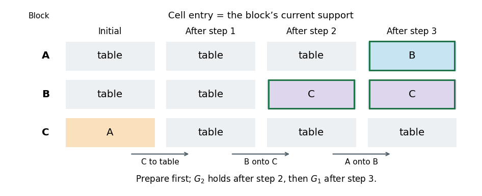
The green-outlined cells mark achieved goal facts. This original solution timeline makes the distinction explicit: independent goal-directed subplanning fails, but unrestricted concatenation does not. To obtain the intended impossibility claim, “non-interleaved” must also forbid anticipatory preparation or require the isolated subplans described above. No source input is missing; the issue is the breadth of the printed definition.

Use a sequential SATPlan encoding with times $t=0,\dots ,T$. The fluent universe isThere are nine support Boolean variables and three clearance Boolean variables per time layer. Static block types, parameter inequalities and permanent table availability are handled during action grounding. For each well-typed ground action $a$ from parts (b)–(c), introduce an occurrence Boolean variable $a_t$ for $0\le t<T$. Allow at most one action per layer, including no action, so that a horizon of $T$ encodes at most $T$ physical actions.

The complete initial-state formula isEvery well-typed fluent not initially true is explicitly false. The final goal formula is simply $G_T=\mathrm{On}(A,B{)}_T\wedge \mathrm{On}(B,C{)}_T$. Leaving unrelated final facts unconstrained is appropriate; leaving unrelated initial facts unconstrained would introduce imaginary starting states.

For each $t<T$, include all action precondition axioms $a_t\to {\bigwedge }_{p\in \mathrm{Pre}(a)}{p}_t$, after removing static true conditions. For example,The precondition axiom for $\mathrm{MoveToTable}(C,A{)}_t$ similarly requires $\mathrm{On}(C,A{)}_t\wedge \mathrm{Clear}(C{)}_t$.

For every fluent $p\in \mathcal{P}$, let ${\mathrm{Add}}_p(t)$ be the logical disjunction of actions at $t$ adding $p$, and ${\mathrm{Del}}_p(t)$ the logical disjunction deleting it. Include the successor-state axiomIt combines action effects with the frame axiom, preventing unsupported changes. A fully grounded example isApply the same construction to every support and clearance fluent, using the exact add/delete lists. If no action occurs, both effect logical disjunctions are false, so all fluents persist.

The sequential action exclusion axioms are $\neg a_t\vee \neg b_t$ for every pair of distinct grounded actions $a,b$. For example,forbids selecting those two occurrences together. Do not add a requirement that some action occur in every layer: that would remove idle padding and change “at most $T$” into an exact-length requirement. One may additionally include true planning state invariants, such as a block having at most one support and a block support carrying at most one block; the unlimited table must be exempt from the latter restriction.

Finally, conjoin $I_0$, $G_T$, and all precondition, successor and exclusion formulas over the layers to obtain ${\phi }_T$. It is a propositional formula; if a solver requires conjunctive normal form, use a satisfiability-preserving Tseitin transformation with auxiliary Boolean variables. The equivalence between this encoding and real action sequences follows from sequential SATPlan correctness: a satisfying assignment induces exactly the stated STRIPS trajectory, and every sufficiently short valid plan supplies such an assignment.

Read the satisfying assignment in increasing time order. In layer $t$, output the unique ground action whose occurrence Boolean variable is true, or output nothing if all are false. Discard idle layers. The result is a sequence of at most $T$ actions.

For correctness, the layer-zero planning fluents are exactly the actual initial state. The action precondition axioms make the selected action applicable, while the successor-state axioms give precisely its add/delete update; the action exclusion axioms prevent simultaneous competing actions. By induction, every following time layer is the real state reached by the decoded prefix. The final goal formula therefore proves that the extracted plan reaches both required goals.

Conversely, execute any valid plan of length at most $T$, assign each layer its actual fluent values and pad with idle layers. These values satisfy every component of ${\phi }_T$. In this instance, decoding the three-action trajectory in part (d) gives a model at $T=3$ and at every larger horizon after padding; direct state-space and propositional checks find no model for $T<3$.