The equilibrium points satisfy and , so they areThe Jacobian matrix and its eigenvalue equation areAt the eigenvalues are , so both points are saddle equilibria. Their stable and unstable tangent directions have slopes and , respectively.
At the eigenvalues are , giving a centre for the linearized equation. Purely imaginary eigenvalues alone do not classify the nonlinear system. The first integral established in part (ii) proves that is in fact a centre equilibrium. It is clockwise: immediately to its right, with and , the vector field points downwards. Thus the final nonlinear classification is
Where , taking the quotient of the two ordinary differential equations givesChoose the first integralThe chain rule checks conservation even at points excluded in taking that quotient:Thus each trajectory is contained in a connected component of a level set of . At the gradient vanishes and the Hessian matrix is the identity, so has a strict local minimum there. To make the closed-trajectory argument explicit, put and . The bounded component of isThe two arcs join at to form a simple closed curve that is a regular level set. The gradient cannot vanish on it: the only critical point of a dynamical system in is the centre, whose level is .
The vector field is tangent and nowhere zero on this compact set, so its speed has a positive minimum. It therefore traverses the curve in finite time and returns to its initial point, giving a periodic orbit. These ovals shrink to the centre as . This is the planar first integral criterion for a centre and proves the required nonlinear assertion; it also gives Lyapunov stability without asymptotic stability.
The nullclines areOn , away from the equilibrium points, the vector field is vertical. Its crossing direction is downwards for , upwards for , downwards for , and upwards for , because . On each of , the vector field is horizontal: it points right when and left when .
Throughout each complementary region, has the sign of , and has the four signs just listed. These signs orient the level sets from part (ii). In particular, the inner periodic orbits are clockwise. The saddle level is , whose separatrices satisfyFor , the upper arc goes from to ; the lower arc goes back from to . These two heteroclinic orbits form a closed boundary around the family of periodic orbits. The remaining branches of the same saddle level extend outwards. The sketch shows the surrounding nonclosed trajectories as well as the nullclines and equilibrium points.
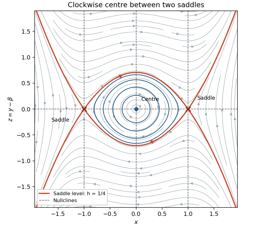
The phase plane in coordinates x and y minus beta, showing clockwise periodic orbits and saddle connections
. Details. 
Set . Then the autonomous planar system becomeswhich has no dependence. ThereforeMore precisely, replacing by sends every trajectory to , with the same time parametrization. The equilibrium points, nullclines, periodic orbits and separatrices all undergo this same translation. Their types and orientations are independent of , so varying produces no bifurcation.
Articles by others on the same topic
There are currently no matching articles.