For zero viscosity, the method of characteristics gives and . On the sloping part of the initial profile, , so . While this map is increasing, inversion givesThe sloping interval shrinks from width one to zero while its height decreases from two to one. Its spatial derivative is and diverges as . Thus the first shock formation by characteristic intersection occurs atFor the profile consists of a left plateau, a straight descending ramp ending at zero, and a right zero plateau. At the ramp becomes a vertical jump. This is a damped Burgers equation; viscosity smooths that jump into a thin transition.
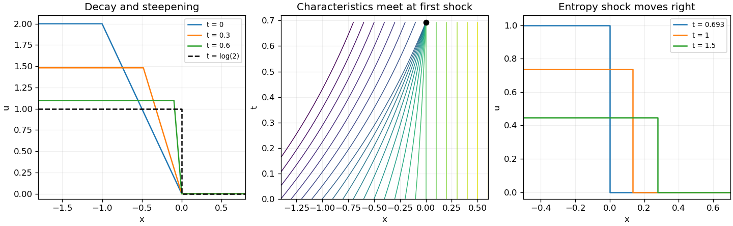
Decay and steepening of the inviscid ramp, its characteristic collapse, and the entropy shock after formation
. Details. 
In the moving stretched coordinates, and . Multiplying the damped Burgers equation by givesDiscarding the order- terms yields the leading Viscous Burgers travelling shock equation . Integrate across a nonconstant transition whose derivative vanishes at either end:Multiplication by and a further integration by parts giveThe first identity is the Rankine-Hugoniot condition, giving . Substitution into the second makes its left side , so the viscosity-selected entropy shock has .
After the first characteristic collapse, the shock is fed by the left constant initial state and the right zero state. Their damped values are and . Therefore . Matching to yieldsThese matching states are consistent with the characteristic feet: the left foot is , while the right foot is . The formula describes the leading thin-layer position in the small-viscosity limit.
Assume a classical solution continuous up to the relevant boundary. At an interior positive maximum, and , hence , a contradiction. At a positive maximum on the top edge , away from the spatial endpoints, the left time derivative satisfies , while again ; the same contradiction applies. Thus a positive maximum can occur only on the initial or lateral parabolic boundary.
For two solutions with the same data, their difference satisfies and vanishes on that parabolic boundary. The weak parabolic maximum principle prohibits a positive maximum of and also of . Therefore , proving at most one solution. The positive reaction term is what gives the immediate strict contradiction at a positive maximum.
Use the Fourier transform convention . Then the equation and Dirac delta initial condition becomeso . The inverse Fourier transform givesComplete the square as and use the permitted complex-shift Gaussian integral. Thus the heat kernel with constant absorption isIts mass is , consistent with constant absorption, and it tends to the Dirac delta as a distribution as .
For a fixed observation point , use the backward adjoint Green function with . It satisfies for , decays with its spatial derivative as , and has terminal distribution . Extending it by zero for gives .
For , integration by parts provesEvaluating this constant pairing at the initial and terminal times yieldsBy translating the heat kernel with constant absorption and reversing the time difference,The terminal singularity is understood as a distribution; the representation follows for smooth decaying data and extends to standard integrable data by the heat-kernel approximation argument.
Differentiate the other parameter. The difference of the required sides isThe first bracket is zero by the prescribed initial compatibility condition, and the second is zero by differentiating . Thus as well. These calculations use the differentiability of the supplied parametric functions.
If the coordinate Jacobian determinant is nonzero, the inverse function theorem gives local coordinates . The chain rule then makes solve a homogeneous two-by-two linear system with determinant . ThereforeThis is the method of characteristics for a first-order equation depending only on the gradient.
Take . Parametrize the initial line by , , . Initial compatibility gives , and then gives . The characteristic formula in part (a) yieldsSince , take . To select the branch connected smoothly to the initial data, stop each characteristic before its coordinate map folds. Its Jacobian determinant isso this branch has . Eliminating givesFor fixed , the right side defining is strictly increasing on that selected branch. At its lower endpoint it equals , and it tends to infinity as . Thus it gives exactly one for every point inSubstituting that unique into the formula for gives the required classical solution. As at fixed , , and as required.
Without the pre-fold branch restriction, the algebraic equation also has a smaller positive root. That root tends to zero as , and its tends to zero rather than , so it does not solve the prescribed initial-boundary problem. The fold is the characteristic caustic; uniqueness here is for the classical branch continued from the given initial data before that fold.
Articles by others on the same topic
There are currently no matching articles.