Original solutions to all six questions and nineteen numbered terminal parts of the Differential Equations and Applications paper sat on 14 June 2011. Source: released Mathematics papers,
Part B 2007 11.pdf. Question 3 distinguishes the conflicting printed Laguerre normalizations. Statements are not reproduced.A distribution is a linear functional on the space of test functions that is continuous in its test-function topology. Equivalently, for every compact there are an integer and a constant such that whenever has support in .
Linearity of follows from linearity of the integral and derivative. Since the integration interval has length ,This is a test-function seminorm estimate of order one, valid for every and even uniformly in . It proves that each is a distribution.
The function is continuous at zero, so its average over tends to its value there. ConsequentlyThe Dirac delta satisfies , and its distributional derivative satisfies . Hence the distributional convergence is
The characteristic polynomial after multiplication by four is , with roots . Thus the general real solution of this constant-coefficient ordinary differential equation isEquivalently the change of dependent variable gives .
In the distribution definition, the Green's function is characterized, for fixed , byIn the classical definition, solve separately for and , with those endpoint conditions, and imposeA jump in would introduce a distributional derivative of the Dirac delta, absent from the right side. Continuity eliminates it; integrating the equation across leaves one quarter of the derivative jump equal to one. These Green function jump conditions make the definitions equivalent. The forced solution is .
Under , the left Robin boundary condition becomes and the right Dirichlet boundary condition becomes . ChooseTheir Wronskian is the constant . For and , it is . The coefficient enforcing the derivative jump four is . Writing and , the Green's function isThe endpoint conditions, continuity and derivative jump follow directly from this Wronskian construction. Its exponential factor also shows why the kernel need not be symmetric in the unweighted inner product.
Put and . Then , so the eigenvalue problem reduces toA nonzero Dirichlet eigenfunction therefore has for an integer . The complete family isThe alternatives give only the zero solution under both endpoint conditions.
The operator itself is self-adjoint with the given unweighted inner product, on the usual regular Dirichlet domain. Indeed , and integration by parts givesfor functions satisfying the endpoint conditions. This is a regular Sturm-Liouville operator with positive leading coefficient , whose Dirichlet realization is self-adjoint. The displayed generalized eigenproblem contains the additional weight ; its eigenfunctions are accordingly orthogonal with respect to , which is separate from the self-adjointness assertion about .
Write asDifferentiating twice, the moving-limit terms cancel at first order and yield at second order. Also and . Thus this integral operator is the inverse of with mixed Neumann boundary condition and Dirichlet boundary condition.
For , satisfies those conditions and . The corresponding mixed homogeneous equation has no nonzero solution, so uniqueness givesThis verifies the asserted eigenvalues and eigenfunctions for every .
Since , the kernel of a linear map is the span of . The self-adjoint Fredholm alternative requires for solvability. If it holds, an arbitrary multiple of can be added, so a solution is not unique.
For ,so case (A) has no solution. For ,by sine-function orthogonality. Thus case (B) has solutions, and they are nonunique.
For , the Fredholm alternative gives a unique solution exactly when for all , unless a resonant problem could exceptionally be compatible. Here none is: with ,At every resonance the compatibility condition therefore fails.
The case must be checked separately because is a compact first-kind integral operator. For every admissible , is continuous and , whereas . Hence has no solution. Combining these cases,In the nonresonant nonzero case the shifted eigenvalues stay away from zero, since and , so inversion is bounded on the Hilbert space.
After division by , the ordinary differential equation has coefficients and . At zero, and , making zero a regular singular point. The indicial equation isso the indicial exponents are , coincident when .
At infinity put and . The transformed equation isThe coefficient of already fails the regular-singularity test at . Thus , including when .
There is a normalization conflict in the source: the printed Rodrigues' formula gives the standard Generalized Laguerre polynomial with , which is generally not one. The norm requested here corresponds to that Rodrigues normalization. A solution normalized to one at zero is .
Set and . The equation becomes . Multiply the equations for by the opposite polynomial, subtract and integrate. The boundary term vanishes at zero and infinity, soThis proves orthogonality for under either normalization.
For the squared norm, use the printed Rodrigues' formula and integrate by parts times:All boundary terms vanish: the required derivatives have a positive power of at zero and exponential decay at infinity. The leading coefficient is , so . The Gamma function integral givesFor the source's alternative unit-at-zero normalization the correct answer instead isBoth cannot equal the printed norm when . This distinction is the normalization of generalized Laguerre polynomials.
For the two normalizations agree, and the Laguerre polynomials are orthonormal with weight . Take real . Their expansion coefficients for the requested function areSubstitute Rodrigues' formula and integrate by parts times. Differentiating transfers a factor after the two sign factors cancel. ThereforeThe integral is by the Gamma function. Boundary terms vanish throughout this range.
The resulting generating function for Laguerre polynomials isOne can also verify convergence and equality directly: Rodrigues' formula gives , and summing reduces the double series to the exponential on the left. The absolute-value double series converges for fixed and , justifying the interchange; the formula then also holds for complex in that disk.
For zero viscosity, the method of characteristics gives and . On the sloping part of the initial profile, , so . While this map is increasing, inversion givesThe sloping interval shrinks from width one to zero while its height decreases from two to one. Its spatial derivative is and diverges as . Thus the first shock formation by characteristic intersection occurs atFor the profile consists of a left plateau, a straight descending ramp ending at zero, and a right zero plateau. At the ramp becomes a vertical jump. This is a damped Burgers equation; viscosity smooths that jump into a thin transition.
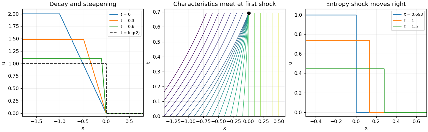
Decay and steepening of the inviscid ramp, its characteristic collapse, and the entropy shock after formation
. Details. 
In the moving stretched coordinates, and . Multiplying the damped Burgers equation by givesDiscarding the order- terms yields the leading Viscous Burgers travelling shock equation . Integrate across a nonconstant transition whose derivative vanishes at either end:Multiplication by and a further integration by parts giveThe first identity is the Rankine-Hugoniot condition, giving . Substitution into the second makes its left side , so the viscosity-selected entropy shock has .
After the first characteristic collapse, the shock is fed by the left constant initial state and the right zero state. Their damped values are and . Therefore . Matching to yieldsThese matching states are consistent with the characteristic feet: the left foot is , while the right foot is . The formula describes the leading thin-layer position in the small-viscosity limit.
Assume a classical solution continuous up to the relevant boundary. At an interior positive maximum, and , hence , a contradiction. At a positive maximum on the top edge , away from the spatial endpoints, the left time derivative satisfies , while again ; the same contradiction applies. Thus a positive maximum can occur only on the initial or lateral parabolic boundary.
For two solutions with the same data, their difference satisfies and vanishes on that parabolic boundary. The weak parabolic maximum principle prohibits a positive maximum of and also of . Therefore , proving at most one solution. The positive reaction term is what gives the immediate strict contradiction at a positive maximum.
Use the Fourier transform convention . Then the equation and Dirac delta initial condition becomeso . The inverse Fourier transform givesComplete the square as and use the permitted complex-shift Gaussian integral. Thus the heat kernel with constant absorption isIts mass is , consistent with constant absorption, and it tends to the Dirac delta as a distribution as .
For a fixed observation point , use the backward adjoint Green function with . It satisfies for , decays with its spatial derivative as , and has terminal distribution . Extending it by zero for gives .
For , integration by parts provesEvaluating this constant pairing at the initial and terminal times yieldsBy translating the heat kernel with constant absorption and reversing the time difference,The terminal singularity is understood as a distribution; the representation follows for smooth decaying data and extends to standard integrable data by the heat-kernel approximation argument.
Differentiate the other parameter. The difference of the required sides isThe first bracket is zero by the prescribed initial compatibility condition, and the second is zero by differentiating . Thus as well. These calculations use the differentiability of the supplied parametric functions.
If the coordinate Jacobian determinant is nonzero, the inverse function theorem gives local coordinates . The chain rule then makes solve a homogeneous two-by-two linear system with determinant . ThereforeThis is the method of characteristics for a first-order equation depending only on the gradient.
Take . Parametrize the initial line by , , . Initial compatibility gives , and then gives . The characteristic formula in part (a) yieldsSince , take . To select the branch connected smoothly to the initial data, stop each characteristic before its coordinate map folds. Its Jacobian determinant isso this branch has . Eliminating givesFor fixed , the right side defining is strictly increasing on that selected branch. At its lower endpoint it equals , and it tends to infinity as . Thus it gives exactly one for every point inSubstituting that unique into the formula for gives the required classical solution. As at fixed , , and as required.
Without the pre-fold branch restriction, the algebraic equation also has a smaller positive root. That root tends to zero as , and its tends to zero rather than , so it does not solve the prescribed initial-boundary problem. The fold is the characteristic caustic; uniqueness here is for the classical branch continued from the given initial data before that fold.
Articles by others on the same topic
There are currently no matching articles.