In the non-scattering grey atmosphere approximation, is the frequency-integrated specific intensity along a ray, is distance along that ray, is the mass density, and is the mass absorption coefficient. The local thermodynamic equilibrium source is the frequency-integrated Planck function . Across a thin element , absorption removes and thermal emission adds . Their balance gives .
Take the upward vertical as the polar axis, put , and define downward optical depth byAlong a ray, and . The chain rule therefore gives . In a plane-parallel, azimuthally symmetric field, the solid angle element is , soLocal radiative equilibrium requires zero net radiative heating of the material: absorption balances emission . Where the absorption coefficient is nonzero this gives , and substitution gives the required angular radiative transfer equation. It does not require the specific intensity itself to be isotropic.
At the top of an atmosphere with no external incoming long-wave radiation, impose . These are inward directions; prescribing the same zero value for outward directions would remove the emergent radiation as well. The upward radiative flux and its derivative areThus : local radiative equilibrium expresses energy conservation through successive atmospheric layers.
The first Saint-Venant equation conserves water volume. The second balances material acceleration against downslope gravity, bed friction and the free-surface pressure gradient. With length scale , depth scale , slope and velocity scale , the conventional gravity-friction scaling has and Froude number . The pressure-gradient/downslope-gravity ratio is , and the inertia/downslope-gravity ratio is .
The uniform steady solution obeys and , hence . In the constant-flux river momentum relaxation reduction, substitute and . Since and , the resulting quasilinear partial differential equation isA downstream boundary at supplies data into precisely when , equivalent to . Although water flows out there, the relevant characteristic curves carry information upstream in this subcritical regime.
Along a characteristic curve, and . Positive relaxes toward ; near , its displacement decays at rate . Boundary-generated deviations therefore become small after a time of order and, while the characteristic speed stays bounded away from zero, within a distance of order . The outer state is the initial uniform solution. A jump between initial and boundary values at their corner can produce a weak solution or a thin initial adjustment; a globally smooth corner solution requires compatible data.
For the moving boundary put . The characteristic speed relative to it is , while the outer speed isFor the intended tidal slowing , is decreasing in and hence throughout the relaxation. Thus leaves an incoming family and an attached thin boundary layer. The diagram shows numerical characteristics of this scalar reduction, with a slower boundary velocity. When , the tidal boundary overtakes the unperturbed characteristic family; an attached smooth relaxation layer is no longer appropriate, and a tidal bore or shock wave can arise in a fuller river model.
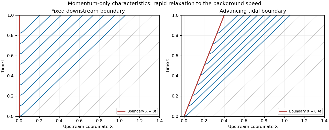
Characteristics leaving a slowly advancing tidal boundary
. Original calculation for the scalar momentum reduction, with , , , and . Curves approach the background characteristic speed after a short relaxation; this is not an exact solution of the full mass-and-momentum system. Details.
There are two qualifications to the printed reduction. First, without the physical slowing assumption, alone need not make the boundary incoming: for , also require . Second, imposing exactly everywhere in the original continuity equation gives , and consequently . The time-dependent characteristics above solve the requested momentum-only approximation, rather than the complete Saint-Venant equation system with an exactly constant flux.
Bedload transport carries sediment by rolling, sliding and short hops near the bed. Suspended sediment is held in the water column by turbulent mixing. The competition between particle settling velocity and the turbulent vertical velocity scale chiefly determines which description applies; particle size and density influence that settling velocity.
Scale the depths and bed/free-surface elevations by , both velocities by , distance by , and time by . A choice producing exactly the requested coefficients isThe sediment continuity equation then has unit coefficients, while both material-acceleration time derivatives acquire the factor . Dividing water momentum by and sediment momentum by givesFor example , , , and give and . These are illustrative values: small effective mobile-layer thickness and small slope explain the two small parameters.
Set at leading order. Water continuity gives , with spatially constant flux; take a prescribed constant . Water momentum integrates to . Since ,The bedload transport model with sediment inertia has remaining equations and .
Choose a uniform state of this reduced model with , constant , andIt satisfies . For small perturbations of the two velocities, put and . Linearization givesFor a Fourier mode this yieldsEvery nonzero mode decays for and grows for . The spatially uniform mode is neutral, and is a singular threshold where the neglected terms matter. In a general uniform state the controlling sign is : equivalently the actual mean-flow Froude number is less or greater than one. The displayed criterion uses the stated unit-depth, unit-velocity normalization of the reduced steady state.
Basal sliding allows ice to pass over bed obstacles by enhanced deformation and regelation: pressure-induced melting on the upstream side and refreezing downstream transfer ice around small obstacles. Cavitation opens water-filled gaps on the downstream side. Their size and the remaining ice-bed contact depend on effective pressure in subglacial drainage as well as basal shear stress . At fixed , reducing generally enlarges cavities and reduces resistance, giving a sliding law with in this regime.
A linked cavity drainage system connects these cavities through passages along the bed. Under the prescribed decreasing relation , the chain rule gives . This conclusion uses that hydraulic relation; it need not apply to a different drainage regime.
With , the ice continuity equation becomes . For bounded spatial gradients over , is independent of the fast seasonal time to leading order. Meanwhile gives , soLet . Direct differentiation proves thatsatisfies the equation and . This is the boundary-generated solution, or a periodic-forcing solution with the forcing continued into its past. An independently prescribed initial profile would also need matching in the region whose characteristic curves have not yet reached the upstream boundary.
If , is invertible and rearranging gives . For with ,Substitution, followed by the sine-difference identity, givesFor fixed and nonzero first-order amplitude, the extrema occur at . Since , the seasonal phase lag in linked cavity drainage gives the stated phase relation . Maxima and minima alternate; when , the first-order approximation is flat and does not locate individual extrema.
Articles by others on the same topic
There are currently no matching articles.