This combined University of Oxford Part C paper covers Mathematics and the Environment in section A and Mathematical Physiology in section B. The original archive transcription retains all seven printed pages and formal identifiers. [ref]
https://www.whatdotheyknow.com/request/maths_past_papers_3. Source release
Bounded official-source searches found no advertised answers for this exact paper. The solutions distinguish valid asymptotic conclusions from the printed claims that require additional assumptions.The heat capacity per unit horizontal area is : mass density times specific heat capacity times atmospheric depth. Thus is the rate of stored thermal energy per unit area. The solar constant is the incident radiative flux on a surface normal to sunlight; the ratio of the Earth's intercepting disk area to its spherical area is . The absorbed fraction is , where albedo is the reflected fraction. The outgoing radiative flux is , a Stefan–Boltzmann law with effective radiation factor incorporating the simplified greenhouse effect. Every term therefore has units of power per area.
The albedo curve decreases smoothly, passes through , and approaches at high temperature. At it is , close to when is large. Its derivative isAn ice-covered planet reflects more sunlight than exposed land or ocean. Warming removes reflective ice, lowers albedo, and increases absorbed radiative flux: this is ice-albedo feedback. The parameter controls the sharpness of this transition; the formula is an idealized global response, rather than a local melting law.
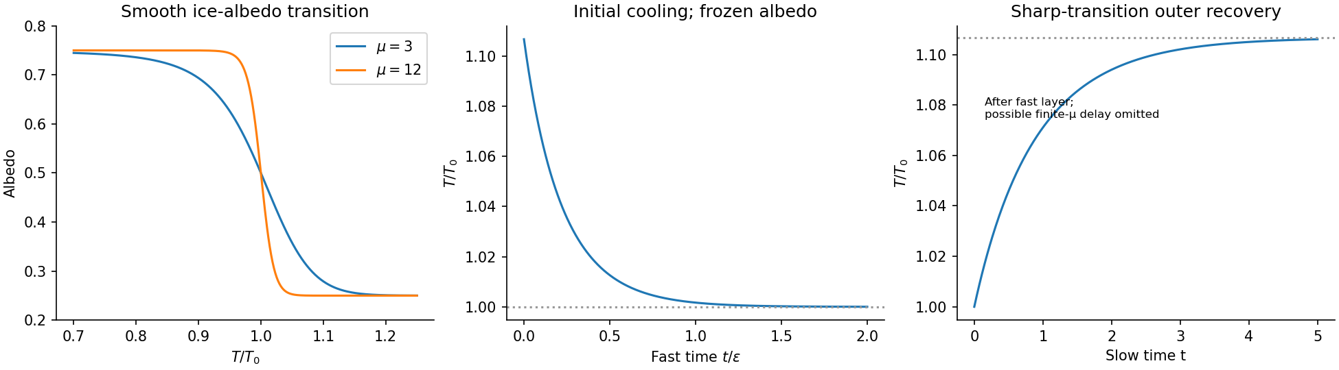
Temperature-dependent albedo and the separated fast cooling and slow recovery
. Details. Set . Since , the steady state energy balance is . Substitution givesThe two sides have slopes and at the origin. For , is strictly concave, its initial slope is , and it remains below . Consequently no positive root exists for , while for there is exactly one positive root . Oddness supplies the corresponding negative root. At the only root is still zero. Hence multiple steady temperatures occur precisely when .
The largest root corresponds monotonically to the largest positive absolute temperature:For large , the positive root tends to , so and . The negative branch has larger albedo and lower temperature.
Use dimensional quantities and set , . Dividing the energy balance by and the albedo equation by its time scale givesThus is the ratio of the atmospheric thermal response time to the much longer albedo response time. Converting kilometres to metres and years to seconds gives , , , andThe thermal time is about half a year, compared with a millennium for albedo adjustment. This is a singular perturbation: setting removes the independent initial condition for temperature.
Initially and , so . On the fast time , albedo changes by only andThus temperature rapidly falls towards . At the same time while , which seeds selection of the warm branch. Afterwards the approximate slow manifold is : decreasing albedo makes temperature rise slowly back towards . The preceding figure separates these two time scales; a single time axis would compress the initial fall into a nearly vertical segment.
In the sharp-transition regime, after selection of the warm branch . Solving the linear ordinary differential equation with the leading matched value givesThese are outer solutions: their initial temperature is , so the fast cooling layer is required to satisfy the actual initial temperature.
There is a useful qualification to the two-limit argument. For fixed finite , put on the slow manifold. Then , and is an unstable equilibrium with growth rate . The small positive seed from the fast layer can therefore produce a delay of order . The simple exponential approximation assumes that the sharp albedo transition is sufficiently fast to make this delay negligible on the displayed slow scale. It is not a uniform approximation for every fixed as .
Assume constant mass density, a prismatic channel, approximately uniform cross-sectional velocity , a hydrostatic pressure distribution, small bed slope , and no lateral inflow. Integrating mass conservation over a slice of length gives , hence .
Let be the hydrostatic first moment, where is the actual free-surface depth. The downstream momentum balance isUsing reduces its left side to . For a fixed prismatic cross-section, , so . Therefore the exact depth-averaged result isHere hydraulic radius converts perimeter shear stress into force per unit fluid volume. The printed notation yields the requested equation if it denotes this hydraulic pressure head, whose derivative equals .
The geometrical definition printed in the next part needs care. Triangular-channel hydrostatic pressure head gives the factor explicitly. For the stated symmetric triangular notch, the actual depth is , whereas its printed is . Indeed and , giving . Thus the equation with precisely the printed geometrical has pressure term . A first-principles derivation cannot remove that factor. The subsequent intended scaling can be carried out algebraically using the printed convention, as below, or with the pressure scale doubled for the actual triangular channel.
Write , , where the given geometry givesTake a Chézy drag law and restrict to downstream flow . Choose an area scale , length scale , and speed scale satisfyingThis makes gravitational driving and drag equal in the reference uniform steady flow. Dividing the printed momentum equation by givesMass conservation retains . In this notation is the square of the velocity-to-gravity-wave-speed ratio based on the chosen depth scale; authors sometimes instead denote its square root by Froude number. If the actual triangular pressure head from the preceding solution is used, replace by in both parameter definitions. The displayed dimensionless form remains the same, with consistently redefined parameters.
First neglect inertia relative to the pressure correction, requiring for smooth fields on these scales. The positive velocity isMultiplying by area gives the discharge . HenceThe leading equation is a nonlinear kinematic wave equation. The pressure correction has positive diffusion coefficient for and smooths steep gradients. Dropped terms are and inertial terms on the assumed scales; sufficiently thin fronts require a separate balance rather than an unrestricted Taylor expansion.
Let the original area be and the increased upstream area be . At , the conservation law flux is strictly convex. Characteristics behind the increase travel faster than those ahead, forming an admissible shock wave. Rankine-Hugoniot conditions give its speedAt the idealized hydrograph jumps from to at . With positive , the diffusion term spreads the rise over a finite interval. The hydrograph is rounded, with an earlier small response and a later approach to the new discharge, rather than an instantaneous jump.
The physical cause is the longitudinal pressure gradient: a local increase in depth influences neighbouring sections and redistributes water before pure downstream transport would deliver a discontinuity. For a small increase, linearization about has speed and diffusivity . The smooth curve in the figure is the exact half-line step response for this linearized advection-diffusion equation; it illustrates the shape without claiming to solve a large nonlinear jump exactly.
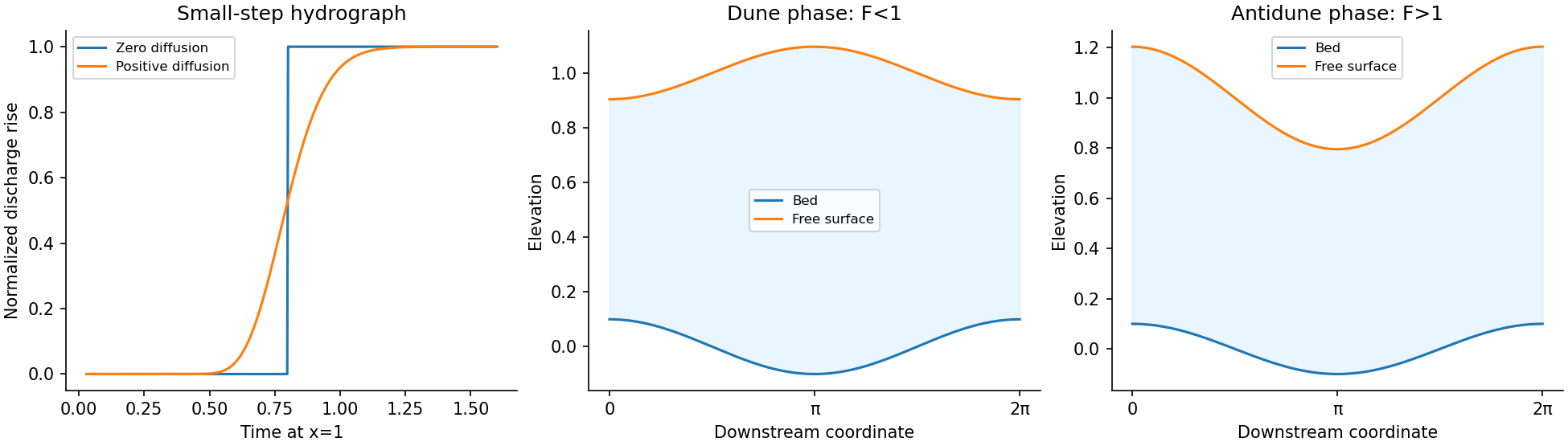
Sharp and diffused downstream hydrographs, with subcritical and supercritical bed-surface phases
. Details. The water mass conservation equation inherited from the earlier model is . It is essential: without it the printed displayed equations are not closed. Take the slow bed branch , and perturb the uniform state by , , , and . For , mass conservation gives and .
Put ; the extra comes from linearizing . The linearized momentum and suspended-sediment equations areEliminating gives the dispersion relationAway from , for fixed nonzero and negligible ,Thus growth requires . For , any gives an unstable branch; for growth would require . A physically increasing erosion function therefore gives the supercritical instability in this simplified model, rather than proving growth of ordinary subcritical dunes. Retaining drag giveswhich shows its stabilizing correction and the need to reconsider the limit near critical flow.
The negative bed-to-surface ratio for subcritical flow means bed crests lie beneath surface troughs: the dune phase relation. Its positive sign for supercritical flow gives aligned crests: an antidune. In the unstable supercritical case the imaginary part gives upstream migration, since . The figure shows these two phase relations. They identify the bedforms but do not by themselves establish growth. The qualitative limitation of the suspended-sediment mechanism is also discussed in the official [ref]
https://people.maths.ox.ac.uk/hewitt/publications/C5_11_notes.pdf. Mathematical Geoscience notes, pages 41–42
.Resolve gravity into components down the bed and normal to it. For slow incompressible flow, inertia is negligible and Cauchy momentum equation reduces to the divergence of the stress tensor plus the gravitational force density being zero. Write the dominant shear component as and the leading normal stresses as .
The shallow-ice approximation assumes a small thickness-to-length ratio. Vertical variation of the shear is retained in the along-bed equation, while longitudinal deviatoric-stress gradients and the shear contribution to the normal equation are higher order. The leading balances are consequentlyThe second is a hydrostatic pressure balance; the first balances gravitational driving and the surface-induced pressure gradient against vertical shear. This approximation requires shallow geometry and sufficiently slow flow, not a Newtonian constitutive equation for ice.
Measure pressure relative to atmospheric pressure. At leading order the stress-free upper surface gives , . Integrating the normal balance first yieldsAt fixed , . Therefore , independent of . Integrating from to givesThis is linear in , is zero at the surface, and reaches its basal value at . In particular the surface slope modifies the shear driving; a flat upper surface relative to the horizontal eliminates it in this approximation.
Set . For downstream shear , Glen's flow law and the no-slip boundary condition giveHere is the ice rate factor, distinct from the cross-sectional area in the river problem. Integrating this velocity profile through the thickness gives the volume flux per unit valley width:The factor combines the depth-dependent shear stress, integration to obtain velocity, and integration to obtain flux. If reverse shear is admitted for noninteger , the signed version of Glen's flow law is ; the displayed unsigned power presumes the downstream regime.
A typical net ice accumulation curve decreases downstream: snow gain at high elevation, zero at the equilibrium line, and negative values in the ice ablation zone. In a steady glacier with zero volume flux at its head, . If its terminus also has zero volume flux, a natural glacier length is the positive root of , with the integral positive between the endpoints. Such a root requires a suitable given accumulation profile; it is not guaranteed by dimensional analysis alone.
Let be a representative accumulation rate and . ChooseUsing , , , , , both terms in mass conservation have scale . The dimensionless flux isDropping hats gives the required partial differential equation. The parameter measures the surface-thickness slope correction relative to the bed slope. For the linear example , accumulation changes sign at and its integrated balance vanishes at .
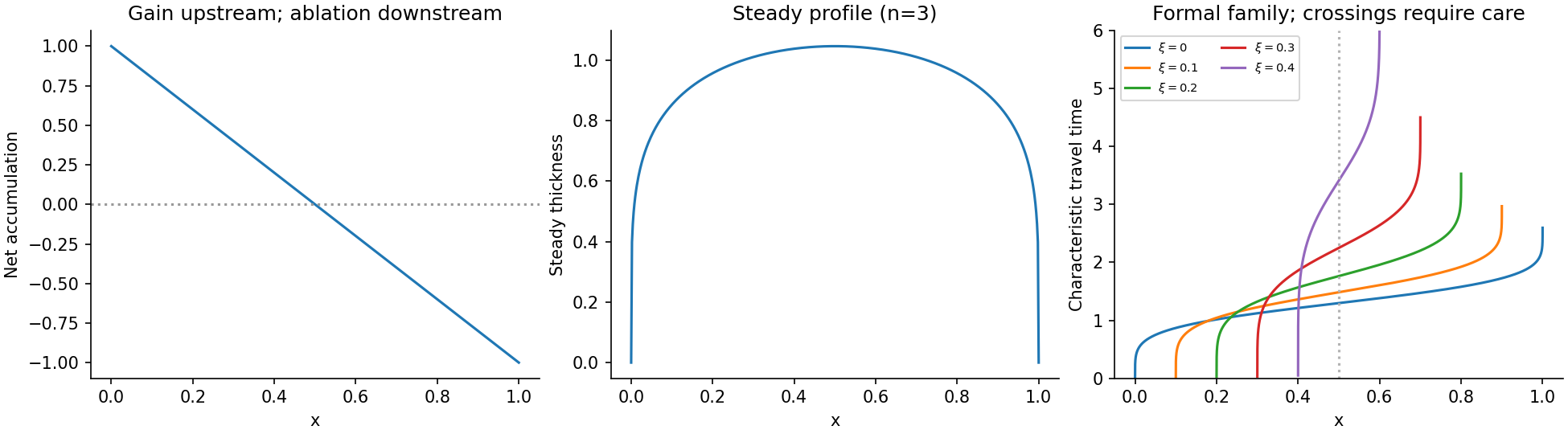
Write , and . Integrating the steady mass conservation equation from the head givesFor the time-dependent first-order equation , method of characteristics gives and . Consequently . On a characteristic starting at with zero thickness,On a characteristic emitted by the boundary , the invariant is zero and . The travel time of the one emitted at time zero isThe incomplete beta function is finite at both endpoints because for the physical exponents . Before characteristic crossings, the initial-data branch and boundary-data branch have the displayed forms in the source, with the appropriate emission time for the latter.
Glacier characteristic admissibility gives a substantive domain restriction. Factoring the invariant gives . A positive forward branch requiresEquivalently it is the image of this parameter domain under , restricted further to regions where that map is single-valued. Characteristics cannot start with positive thickness growth at , where the prescribed initial rate is negative. This is why the printed piecewise expression is a formal characteristic construction, not a global nonnegative solution from a bare bed. For example for , putting givesBoth factors increase with there, so no positive initial-data branch exists at that for , contrary to a literal global reading of the first case. Compression can also make characteristics intersect; entropy solutions then require shock waves.
One can nevertheless give the exact zero-thickness endpoint locus of these formal characteristics. Let . At the change of variable givesThis is the formal snout locus inferred from the given characteristic family; it retreats from towards . It is not justified as the physical terminus of an accumulating glacier formed from zero initial ice. In particular it says nothing about a positive advancing snout at . A physical free boundary problem must specify no ablation on a bare bed, maintain , and select an entropy solution or retain the small slope regularization. Those additional conditions are absent from the printed first-order construction. Thus a unique global physical snout trajectory cannot be claimed from that construction alone. The steady endpoint remains . The degenerate limit would instead have the same endpoint time for every initial characteristic, so the inverted formula presumes .
Use for concentrations and define net complex-formation rates , with . The law of mass action givesEach binding event removes one free substrate molecule; each unbinding returns one; each catalytic event releases one reaction product and reduces the number of occupied sites by one. Suitable initially unbound enzyme and substrate data are , , , for . All rates are nonnegative on the boundary of the nonnegative concentration region in the direction required to preserve it. These equations also conserve , accounting for bound substrate as well as free substrate.
Adding the ordinary differential equations for all enzyme states makes the net rates telescope:With initially unbound enzyme, this sum is for all time. HenceThis is enzyme conservation, not conservation of each complex individually. The reaction changes site occupancy and makes reaction product, but no event creates or destroys an enzyme molecule.
Besides the stated scales, set , , , , and . Then , and direct substitution, remembering , givesThe exact initial values are , , , for . The enzyme-state equations carry the small parameter because the enzyme concentration scale is small relative to the initial substrate concentration; the substrate evolves on the chosen slower depletion time scale.
For an outer solution with bounded derivatives as , the final complex equation gives . Working backwards in then gives every , including ; setting only their sum to zero would not suffice. This is the quasi-steady-state approximation, valid after the initial complex-formation layer with the relevant dimensionless rate parameters held fixed.
The recurrence is , where . Thus , . Substitution into enzyme conservation yieldsEach state produces reaction product at rate , soThe source's uppercase in the index range is read as the number of binding sites. This approximation preserves the total enzyme population and the different catalytic rates of the occupied states.
The sequential-enzyme Hill limit uses the intended distinguished limit for holds the other rates fixed while , , and tends to a positive finite constant. Then for every , , whereas remains finite and nonzero. Hence intermediate complexes have negligible occupancy relative to the unbound and fully bound states.
In the quasi-steady-state approximation rate, all intermediate numerator and denominator terms disappear. Multiplying by givesThis is the Hill equation with maximal rate and effective half-saturation concentration . Here its power follows from the sequential binding mechanism and the suppression of intermediate states.
The phrase “ finite” needs this scaling interpretation for a nontrivial limiting rate. Merely bounding that product, while permitting unrelated rates to vary, does not ensure that all intermediate weights vanish relative to the terminal one. The derivation explicitly supplies the usual fixed-other-rates, positive-product assumptions. For , the rate in the box is already the exact one-state quasi-steady-state approximation rate, without this two-endpoint limiting argument.
Write , and . Since , the exact equations areAt the prescribed initial data , , rather than zero. The quasi-steady-state approximation would instead demand , giving . This mismatch signals an initial layer.
Set and expand , . At leading order , so , while and . ThusFor a more informative substrate approximation, integration of with givesOn the slow scale and , with matched leading value . Integrating gives . In the overlap , the inner complex tends to and its substrate slope matches the expansion of this outer solution. A leading composite asymptotic expansion isIt satisfies both initial values at leading order and smoothly joins the initial complex build-up to substrate depletion. The displayed inner substrate term records the small binding-induced initial slip if greater accuracy is wanted.
The nullclines are the cubic and the straight line . At an equilibrium either , or . The latter quadratic has maximum , so leaves only the resting state . Its Jacobian matrix isBoth eigenvalues have negative real parts; the rest state is linearly stable and asymptotically stable.
On the fast time , the recovery variable is approximately fixed. At , the scalar fast equation has stable roots and an unstable root . A small kick below decays towards rest; a kick above it moves rapidly towards the right attracting branch. For finite , the threshold is displaced from the frozen root by slow recovery, but the leading threshold mechanism is this unstable middle branch.
After the fast excitation, raises while follows the right attracting branch of the cubic. At its upper fold the branch ends and makes a fast downward jump to the left branch. Recovery then lowers slowly, with a negative undershoot in , before return towards . Thus the action potential time trace has rapid depolarization, a slower high-voltage excursion, rapid repolarization, and slow recovery. On the fast segments scarcely changes; on slow segments and . The figure shows a numerically integrated superthreshold excursion and its time trace, rather than just arrows on the nullclines.
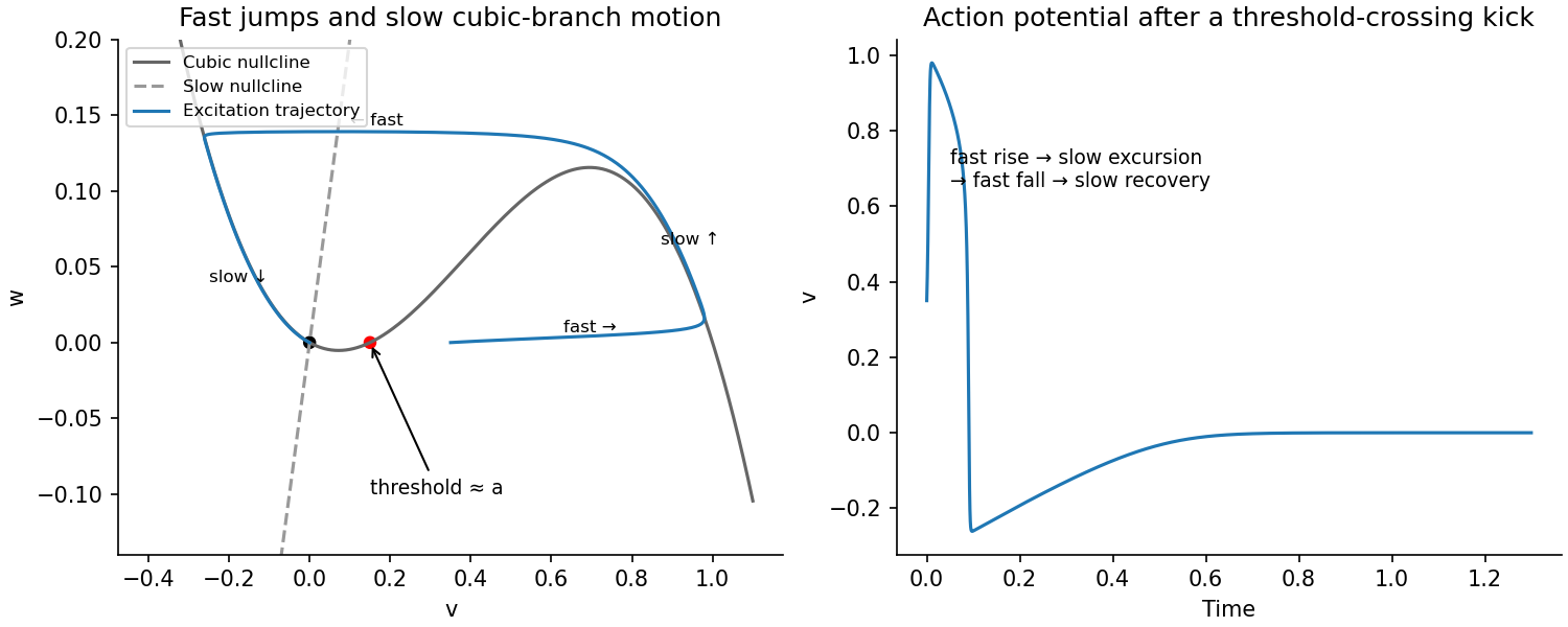
Use . The nullclines become and , while the slow equation becomes . The cubic has foldswith its local minimum and its local maximum. Let and be the left and right attracting roots of . A line whose intersection is on the repelling middle branch permits a relaxation oscillation: upward slow travel on the right branch from to , a fast jump to the left branch, downward slow travel to , and a return jump. For sufficiently large fixed this occurs for currents between the fold values and , away from the small- onset layers. The straight line then crosses each outer branch beyond the relevant slow excursion, so the slow velocities have the required signs.
Neglecting the fast-jump durations, integrate along the two slow segments. Their opposite orientations giveThe printed period omits the current shift. With the source's definition that solve , both denominators must retain in the shifted coordinate. Equivalently, in the physical recovery coordinate the bounds are and the integrand uses . The printed formula is therefore not the leading slow period for the displayed equations unless its notation is changed or an additional approximation justifying the omitted term is supplied.
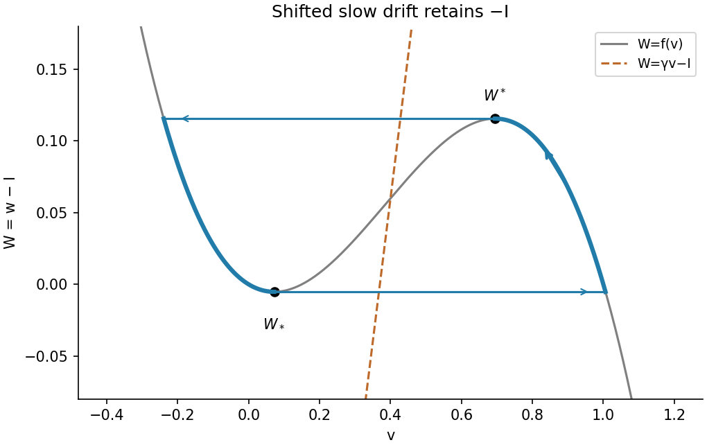


For the chain rule gives , , . ThusAs increases from the material ahead of the wave towards that behind it, the singular pulse construction is . The front raises at approximately fixed from the low root to the high root. On the plateau , on the right attracting branch while rises slowly. The back decreases at approximately fixed to the left attracting branch. The recovery tail then lowers back to zero on that branch, returning to . Both sharp transitions have thickness in ; the other segments have the slower recovery scale.
The figure labels all four points and the front/back orientations. This frozen-recovery construction needs as well as if is large, so that the recovery variable remains nearly fixed in an inner transition. It also needs an admissible positive front speed for the chosen orientation, addressed below.
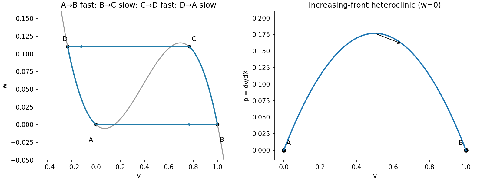
Matched front, plateau, back and recovery tail, with the inner front heteroclinic orbit
. Details. 
Put . The travelling equations become and . Hence, for nonzero speed and , is constant to leading order across the front.
Writing gives the planar system , . At the outer cubic roots and , . The Jacobian determinant is , so both are saddle points. The increasing front is a heteroclinic orbit from the unstable manifold of to the stable manifold of . Varying supplies the shooting parameter required to match these manifolds. For this cubic one can also construct it explicitly, as in the next solution.
Multiply the second-order equation by and integrate across the front. Because at both ends, the term vanishes. The remaining identity isThe denominator is positive for a nonconstant front, so its direction is determined by the signed area between the cubic and the horizontal recovery line: Maxwell balance for a scalar reaction-diffusion front gives zero speed when that area vanishes.
The derivative in the denominator must use the inner coordinate . If one instead uses the source's original and denotes , then and the identity is . Thus the printed is valid only if has silently been reused for the rescaled inner coordinate; with the original coordinate it misses a factor .
Let denote the increasing-front speed from the preceding solution. Reversing that heteroclinic reverses its speed, so a decreasing back has speed . A rigidly travelling pulse has one speed throughout, requiringThis is the correct use of the integral formula: compare the oppositely oriented transitions, including their signs, rather than equating two increasing-front speeds.
For completeness, write , . The explicit increasing frozen-recovery cubic front isSubstitution, using , verifies the equation. Since , speed matching givesFor this selects the appropriate positive back level within the cubic's three-root range. The high branch connects to slowly, and the low branch supplies recovery after .
The stated positive-speed, rising-front orientation imposes at leading order. The printed range by itself does not guarantee that pulse construction: at the leading front is stationary, while for the calculated increasing-front speed is negative. Existence and stability of a full finite- pulse also require the slow connections; speed matching is its leading necessary construction, rather than a proof for every parameter in the printed range.
The common vector field represents an identical reference cell. The small cell-specific term represents heterogeneity of cellular properties, such as differing ion-current parameters or intrinsic oscillation rates. It is not external random noise: the displayed model is deterministic.
The Kronecker delta factors restrict coupling to the first state component, the membrane potential. Substitution gives a coupling current in the voltage equation proportional to , while the other state components have no direct intercellular coupling. This is the linear voltage-difference response of gap junctions. Gating and chemical variables can still change indirectly through their own coupled intracellular dynamics. The zero diagonal removes self-coupling, which would contribute zero anyway. Physical reciprocal gap-junction coupling is often symmetric, but zero diagonal alone does not impose reciprocity; that distinction matters in the final part.
With , , the multiscale chain rule gives . Expanding gives at order oneAt order , moving the linearized reference dynamics to the left givesThe component sum runs over the state variables; the source uses in its first displayed sum and later. All functions for the solvability calculation are periodic in with period one.
Differentiating the autonomous cycle equation gives , so lies in the periodic null space of . For a hyperbolic attracting limit cycle, its tangent direction has Floquet multiplier one and every transverse multiplier has modulus below one. Hence it is the only periodic direction, proving the required one-dimensional null space.
Strictly, mere nonlinear stability does not ensure this spectral assertion. In polar coordinates , has an attracting unit-period cycle but neutral radial linearization at , supplying a second periodic solution of the variational equation. Thus the intended phase reduction assumes the usual simple unit Floquet multiplier, or equivalently hyperbolic transverse attraction; this assumption is made explicit here.
Use the period-one inner product . Periodic integration by parts gives . Let span this adjoint null space and normalize . For oscillator , write . Then and .
The Fredholm solvability condition makes the forcing in the order- equation orthogonal to . Its intrinsic and frequency terms integrate to , whereVoltage-only coupling contributesThus withthe complete phase equation isPeriodicity makes these formulae independent of the absolute initial phase. The adjoint function is a phase response function; it projects a small perturbation of each state component onto its accumulated phase change. The subtraction of ensures zero coupling between identical phases, as required by the original voltage differences. The source's reference to its equation (1) is read as the uncoupled cycle equation, numbered (3) on the actual page.
At a locked state choose the rotating frame with . For small phase differences, Taylor expansion gives . Let the graph Laplacian have and for . The leading locked equations areIf coupling is balanced, for every , so . Summing over cells cancels all linear coupling terms and givesIn particular symmetric reciprocal gap-junction conductances satisfy this condition. To leading order the collective physical frequency is .
The arithmetic-mean conclusion requires this extra balance assumption. The printed condition alone is insufficient. For a connected directed coupling network let , normalized by . The valid weighted collective oscillator frequency result isFor two cells with , , one has and at linear order. For example gives , rather than , while the locked phase difference is when . This supplies a counterexample with arbitrarily small phase differences. It also identifies exactly why reciprocal coupling recovers the requested mean: the left null space is then spanned by the uniform vector.
This University of Oxford Part C paper combines Mathematics and the Environment in section A with Mathematical Physiology in section B. [ref]
https://www.whatdotheyknow.com/request/maths_past_papers_3. Source release
The archive preserves the complete editable seven-page paper. Bounded searches of official sources found no advertised answers for this exact paper. The solutions distinguish linear and asymptotic conclusions from exact nonlinear claims, and identify the carrier-total typo and small-parameter respiratory approximations.For Röthlisberger channel drainage, is the water-filled cross-sectional area of the subglacial channel, its volume discharge, the mass of ice melted per unit channel length per unit time, and the effective pressure, namely ice overburden pressure minus water pressure. The first balance converts melt mass to area growth through division by ice density , and subtracts material creep closure . The cubic pressure dependence comes from the adopted ice-flow law; includes its material and geometric factors.
The second relation balances the downslope hydraulic driving gradient against the adopted frictional pressure loss. It is an instantaneous discharge-area law, giving for positive downstream flow. The final balance equates latent heat needed to melt the channel walls with the gravitational power dissipated per unit length, . It assumes that this dissipated power is available for melting rather than substantial sensible heating or other energy losses. The model thus couples melt opening, pressure-driven material creep closure and hydraulic discharge.
With constant lake surface area, raising its level by changes its volume by . The symbol in the proposed balance is an effective filling rate measured as lake-level rise per unit time, so the volume inflow is . Volume conservation givesThus the lake rises when its inflow exceeds channel discharge and falls in the opposite case. If an inflow were instead specified directly as a volume rate , its contribution would be ; keeping these units distinct is necessary for the interpretation of .
Hydrostatic pressure at the entrance is , with a constant reference pressure. Therefore , and constant overburden pressure givesA filling lake raises water pressure and lowers effective pressure, reducing material creep closure. A draining lake has the reverse effect. These signs supply the pressure feedback in the coupled drainage model.
Write dimensional variables as their scales times dimensionless variables, with positive scales . For compactness defineA consistent explicit choice isThese identities give , , and . Substitution therefore leaves the unit coefficients in all four balances, and the sole supply parameter is . Expanding its scales yieldsAfter dropping scale hats, eliminate the instantaneous quantities to obtain the useful two-dimensional systemThese scales assume a positive slope, positive friction coefficient and nonzero lake area; they nondimensionalize exactly the hydraulic law printed in the source.
For , the positive equilibrium isSet and and retain first-order terms. The linear system isDifferentiating its first row and using the second givesIn particular the trace is positive and determinant is . The steady drainage state is linearly unstable for every positive supply, whether its instability is oscillatory or nonoscillatory.
The characteristic roots satisfyThey are a nonreal conjugate pair precisely when , or . ThereforeIn lake-coupled Röthlisberger drainage instability, above this value the real part is , so nonzero linear perturbations are sinusoidal oscillations with an exponentially growing envelope. Their angular frequency is .
Physically the feedback represents repeated lake filling and pressure increase, channel enlargement by melting, rapid drainage, pressure reduction and material creep closure. Large drainage events are glacial lake outburst floods, or jökulhlaups. The unbounded amplitude is a conclusion of the linearized equations, not a proof of infinite physical discharge or an indefinitely growing nonlinear solution. Once perturbations are comparable with the equilibrium scales, nonlinear dynamics and constraints such as lake depletion must be retained. At the threshold the two real roots coincide; below it the instability is nonoscillatory.
The cross-sectional area multiplied by the mean downstream speed is the volume flux . The term is local storage change per unit river length, is net downstream export per unit length, and is lateral volume input per unit length per unit time, for example distributed tributary or runoff supply.
For a fixed reach , incompressibility and constant density giveApply the fundamental theorem of calculus and localize the resulting integral identity to obtain . The density cancels because every term transports the same water; no sediment source is included in this balance.
To obtain a power-law river kinematic wave, let be the wetted perimeter and the small bed slope. A uniform-flow force balance per unit river length is . With a Chézy friction law , it gives . Thus the hydraulic radius determines the power of area.
For a channel family with , where , we have , with . Set and . ThenFor example a broad fixed-width rectangular channel has approximately constant wetted perimeter, giving ; a geometrically similar channel family has , giving . The exponent is therefore a geometry-dependent consequence of the friction balance, not a universal arbitrary value fixed by Chezy's law alone.
At equilibrium , so for an upstream boundary flux . HenceWithout a specified upstream condition this integration constant must be retained. On a region of positive area, the characteristic speed is , increasing downstream along the equilibrium. Small disturbances move downstream, spread in space as this speed increases, and decrease in area amplitude in the manner derived next. They are transported away from a fixed location; the model has no diffusion giving instantaneous smoothing. Finite-amplitude compressive disturbances can steepen into shocks because the flux is convex, , so the small-disturbance picture is not a global no-shock assertion.
Taylor expansion gives . Subtract the equilibrium equation and write to obtain . Set . Since is time independent, . The travel coordinate for a conservative transport perturbation transforms this into , and thereforeThe conserved quantity along a characteristic is the flux perturbation , explaining the diminishing area amplitude as grows.
Differentiate the equilibrium relation to get . Thus the arrival time is explicitlyFor zero upstream flux the integral remains finite, giving the limiting formula with its second term zero. However then makes the displayed amplitude formula singular at the head; a uniformly small arbitrary area disturbance imposed exactly there is outside this linearization. A positive upstream flux avoids that degeneracy.
Here is water depth, the depth-averaged downstream speed, bed elevation relative to the reference slope, and free-surface elevation relative to that reference. The constants are water and grain densities, is the reference bed slope, bed shear stress, bed porosity, suspended sediment mass concentration, bedload solid volume flux per unit width, and erosion and deposition velocities. The settling speed is denoted by in the constitutive laws.
Depth integration of incompressible water conservation gives the depth-storage plus discharge-divergence balance. Depth-averaged momentum has local and advective acceleration on the left, and gravity driven by the actual surface gradient together with bed drag on the right. Hydrostatic pressure and a shallow-water approximation underlie this Saint-Venant description.
Suspended sediment conservation first has the conservative form ; the water balance reduces it to the material-derivative form printed in the source. Solid bed volume per unit horizontal area is . Its storage plus bedload divergence equals deposition minus erosion, giving the Exner bed balance. Adding the suspended and bed balances after converting bed volume to grain mass cancels exchange terms: erosion and deposition transfer sediment between the two reservoirs rather than create it.
Take an arbitrary reference depth , and select so the uniform reference flow balances drag and slope. Work with positive downstream velocity, so in the dimensional constitutive laws. Introduce the erosion and bedload scalesMatching erosion with deposition, suspended advection with erosion, and bed storage with erosion gives respectivelyUse for the scales of and too, so survives unchanged. After dividing the balances by their matched scales, the parameters areFor example the momentum balance divided by has inertial prefactor , surface-gradient term , and equal slope/drag prefactors , because . The suspended balance has source , and the bed balance has its negative with unit bed-time coefficient by the definition of . These substitutions give the entire stated dimensionless system; is dimensionless bedload, with its dimensional scale already absorbed into .
For quasistatic bed stability with suspended sediment, in the leading approximation, and . For spatially varying perturbations at fixed unit water flux and fixed surface level, write , , , . The constraints give and . Linearizing the suspended and bed equations yieldsFor a Fourier mode , the first relation gives ; substitution into the second givesThus every nonzero spatial frequency has negative growth rate, independently of . The parameter changes propagation, not damping. The spatially uniform mode has and is neutral, representing a change among uniform reference states compatible with the leading constraints. Hence there is no growing linear mode in this approximation; the claim is stability, not strict decay of every homogeneous perturbation. Restoring the small discarded terms or changing boundary conditions requires a separate calculation.
Articles were limited to the first 100 out of 224 total.
Articles by others on the same topic
There are currently no matching articles.