For an experiment beginning by mixing unbound enzyme with substrate, take . The enzyme-substrate complexes, inactivated enzyme and product are initially absent. Nonzero pre-existing product could be allowed without changing the dynamics here, since it has no feedback reaction in the specified scheme.
Write concentrations as in this calculation. The law of mass action assigns the forward bimolecular rate and the first-order rates . Each species gains the rates of reactions producing it and loses those consuming it:Adding the equations for all enzyme-bearing species cancels every reaction rate, so . This is conservation of the total enzyme-derived material, including the inactivated form. It does not assert conservation of active enzyme: mechanism-based inhibition transfers some of that conserved material irreversibly into .
The conserved total is under the chosen initial conditions. Substitute into the equations from the previous part. This closes the subsystem for ; product can be recovered afterward by integrating .
Let and . The required nondimensionalization is completed byIndeed and the free-enzyme fraction is . Substitution and division by the indicated time scale giveFor example explains the coefficient in the third equation. The small multiplier on the intermediate-species derivatives identifies their potentially fast adjustment relative to substrate depletion.
For quasi-steady enzyme kinetics at low substrate saturation, the quasi-steady-state approximation is controlled here by , rather than by alone. Even with , taking makes and .
After the initial fast layer , the third equation givesSince , the last equation gives . Starting from , this implies on bounded intervals of the slow time. The quasi-steady second equation then gives . In the first equation,Matching to the initial substrate value therefore yields . The relation is an outer approximation: it does not replace the initial layer needed to reconcile with . Likewise the smallness of accumulated inactivated enzyme has been justified for bounded slow times, not arbitrarily long times.
For the travelling wave coordinate , the chain rule givesFast-slow matching for a calcium pulse joins two fast transitions, and , joined by slow portions and . Write the nullcline as . The resting point has , in the leading matched description.
Put . Multiplying the first equation by gives . At leading order, integrate and use , at the start of the front. Together with the second equation this givesThe fast equilibria are intersections of and . As the slope changes, there may be one or three simple intersections, with two distinct intersections at a tangency. At a simple point of the nullcline, , and the sign convention above/below it gives . The Jacobian matrix of the fast system hasFor the usual three-intersection configuration, the two outer points have , hence negative determinant and one positive and one negative eigenvalue: they are saddle points. The middle point has positive determinant; it is linearly stable if and unstable if . Zero trace is a possible oscillatory stability threshold, with a nonlinear classification requiring further information about .
To select the front speed, follow the appropriate branch of the unstable manifold of and vary until it meets the stable manifold of . This is a shooting method for a heteroclinic orbit. Follow the high- slow branch from to ; the falling front obeys the same fast equations with the integration constant anchored at . Choose so that its descending saddle connection reaches a low- point at that same speed. The remaining slow branch returns toward the resting point, completing the matched spike. The construction requires the indicated connections; a nullcline sketch alone does not specify their numerical speed or prove their existence for every possible kinetic function .
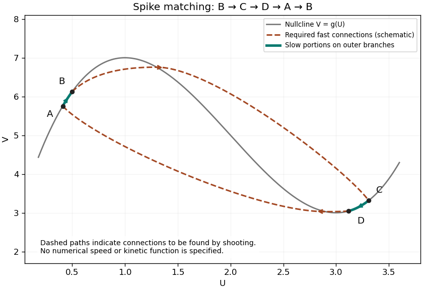
Fast and slow portions of the calcium-wave phase-plane construction
. A qualitative original sketch: the rising nullcline branches carry the slow return and recovery, while dashed paths indicate the saddle connections that a shooting calculation must find. The paths illustrate the matching construction and are not a numerical solution for a specified kinetic function. Details.
On the slow portions, at leading order, so and . Neglecting the small diffusion term yieldsOn the outer rising branches the coefficient on the left is positive. Recovery from toward requires decreasing , hence ; the low branch from back toward rest requires increasing , hence . Therefore . These inequalities distinguish the recovery branches from a trajectory that would move away from the required matching points.
Systole is ventricular contraction and ejection; diastole includes ventricular relaxation and filling. Let denote arterial, venous and left-ventricular blood volumes. Let flow through the aortic valve into the arteries, through the peripheral circulation, and through the mitral valve into the ventricle. Conservation of volume givesThe same leaves arteries and enters veins because the capillary compartment has no changing stored volume in this approximation. Adding the equations conserves total modeled blood volume.
Use constant vascular compliances , with and , and ventricular elastance . The hydraulic resistances and ideal one-way valves givewhere . Substitution into the conservation equations gives the two stated arterial/venous pressure equations. Since , differentiating this identity gives the third equation. The positive parts encode valve closure against a reverse pressure difference.
During isovolumetric contraction both valves are closed. Let be the end-diastolic ventricular volume, its unstressed reference volume, and arterial pressure before ejection. The rapidly raised elastance generates , so the aortic valve opens if .
During ejection, makes the open-valve pressure drop small on the peripheral drainage time scale, so . The mitral valve is closed, and adding arterial and ventricular volume balances eliminates . With this givesFor approximately constant systolic elastance, set and reset time to the start of the slow ejection phase. ThenHere is the matched pressure at that start. If peripheral outflow is negligible during the preceding rapid artery-ventricle pressure equilibration, conservation gives the more explicit .
After aortic closure the ventricular volume is fixed at the end-systolic value . Relaxation decreases until the mitral valve opens at , hence , with the venous filling pressure at opening. During filling the aortic valve is closed, so . With the arterial pressure at the start of filling and time reset there,The change from to is physical: the ejecting ventricle shares the arterial pressure during systole, whereas a closed aortic valve disconnects it during filling.
In this delayed carbon-dioxide ventilation feedback model, is a representative carbon-dioxide partial pressure, an effective storage capacitance, metabolic production, and removal by pulmonary ventilation. The delay represents transport and sensing between the gas-exchange compartment and the ventilatory response. The Hill equation response rises sigmoidally with pressure, reaches half its maximum at , and saturates at ; permits a steep threshold-like response.
For positive parameters, increases strictly from zero to infinity because its derivative is . Its graph therefore intersects the horizontal line exactly once: . The figure shows this argument and the first imaginary-root crossing.
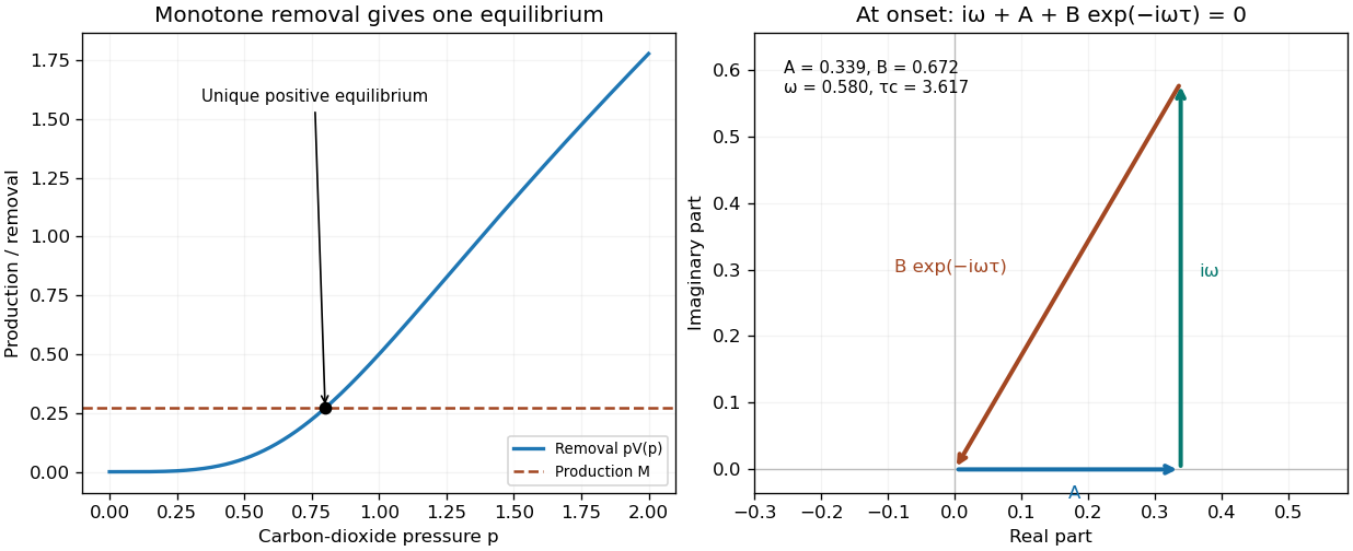

For a small perturbation , linearization givesThe sigmoidal delayed ventilation threshold follows from the characteristic equation of a delay differential equation, . At an imaginary root , separate real and imaginary parts:For , the first positive crossing hasAt zero delay the scalar equation is stable. No root can cross the imaginary axis before this first crossing, and zero itself is not a root. To check the crossing direction, implicit differentiation givesAll subsequent imaginary crossings have the same direction. Thus the equilibrium is linearly stable below and unstable above it. This establishes the oscillatory linear threshold; the full nonlinear Hopf bifurcation additionally requires the usual nondegeneracy conditions. If , no finite imaginary-root crossing occurs and the equilibrium is stable for every finite delay. For the stated response, , showing explicitly when the gain can exceed instantaneous damping.
If , then and . Consequently the small-amplitude period near onset is . The comparison is to the critical delay near the first instability, rather than an arbitrary delay far beyond onset. A longer circulatory transit time can move the physiological system across this delayed-feedback threshold, providing a mechanism for periodic breathing associated with impaired cardiac output.
Articles by others on the same topic
There are currently no matching articles.