It suffices to find a tree component of order . Let count such graph components in the binomial random graph. The Cayley formula and independent edges give the tree-component expectation in the Erdős-Rényi modelHere is fixed. The upper bound on implies , hence andWe first verify that this expected value diverges throughout the permitted interval, including when grows quickly. If , the exponential factor is at least and . If , then . Finally, if , the upper bound on givesThus in all three cases.
For distinct -element vertex sets , write for their tree-component indicators. If they overlap, they cannot both be distinct connected components of a graph, so . If they are disjoint, the absent edges between the two sets are counted twice in the product of their marginal probabilities and once in the joint probability. ThereforeSumming and discarding the negative overlap contributions yieldsThe Chebyshev inequality now gives . Consequently there is a component of order with high probability, in fact a tree component. The argument proves the entire fixed-order tree-component window, rather than only a particular choice of .
Let count -cliques, and put . Since , the Markov inequality gives . Any larger clique contains an -clique, so it remains to prove with high probability.
We give the required growing-clique overlap bound explicitly. Set and, for ,The quantity is the probability that a uniformly chosen -set overlaps a fixed -set in exactly vertices. Two clique indicators share exactly edge requirements, so their joint-to-product ratio is . Overlap zero or one gives independence. Hence the overlap formula for the variance of a clique count impliesWe must bound this sum with allowed to grow.
Eventually and . Using , these inequalities giveFor , a union bound over the selected shared vertices gives . Put . Since and ,For each fixed , the first bound tends to zero if stays bounded, because its power of is negative. If , the middle bound tends to zero because . Thus each fixed- term tends to zero along arbitrary admissible sequences. The bounding series converges. Splitting at a fixed large index, then taking and the index to infinity, proves that the entire lower-half sum is .
For the upper half write . The exact diagonal comparison isFor , the second bound on givesThe last inequality uses : the exponent of in the bracket is negative, so substituting bounds it above. Uniformly for this range of , . Indeed , and concavity of , checked at and , gives . It follows thatThus . The second moment method gives . Combining this with the absence of larger cliques provesThe restriction on is used in both overlap ranges; divergence of a clique count in a binomial random graph alone would not suffice for arbitrary growing .
Couple the uniform random graph process by giving every possible edge an independent uniform label in and revealing them in increasing order. The graph at label threshold is a binomial random graph. Define as the first step with no isolated vertices and as the first connected graph. Deterministically . We prove the reverse inequality with high probability by tracking the same process through a short interval.
Put , , and . At the isolated vertex count hasThe variance estimate follows by comparing two isolated-vertex indicators, whose joint-to-product probability ratio is . Thus with high probability. Also the Markov inequality gives with probability tending to one.
At this same threshold, exclude every graph component with order . For , any such component contains a spanning tree. The Cayley formula and a union bound therefore giveIn this range the bracket is at most . Summing over gives . For , even the cut-absence bound is enough:The bracket tends to zero, so this range also has total probability . Consequently the graph at consists of one component of order greater than and its isolated-vertex set , where with high probability.
Conditional on the entire graph at , every unrevealed edge label remains independently uniform on . In particular,There are no isolated vertices at with high probability, because their expected value is asymptotic to . On the intersection of these events, each vertex of loses isolation by joining the original large component, never by forming a separate small component with another vertex of . At every step between these two thresholds there is therefore one nontrivial component and some isolated vertices. The final isolated vertex disappears precisely when the graph becomes connected. This proves the connectivity hitting time equals disappearance of isolated vertices result:
For the critical-window probability, let with . For each fixed , the falling factorial moment of the isolated-vertex count isuniformly for such shifts. Apply the Bonferroni inequalities to the zero-count event. Its odd and even truncations bracket by partial sums of . Since , their remainders tend uniformly to zero. Hence . The process equality just proved changes this probability by at most its failure probability. ThereforeThe ratio follows because the denominator is bounded below by ; no convergence of is needed.
The printed second conclusion has the complementary denominator and is false as written. For , the printed ratio tends to . Its denominator is correct for the probability of being disconnected. Thus either remove the leading in the denominator or replace “connected” by “disconnected”; the proof supplies both corrected versions.
Put and . Use the configuration model: give vertex exactly labelled half-edges and choose a uniform perfect matching of all half-edges. There arepairings, with denoting a falling factorial. Each allowed simple graph has exactly representations: at every vertex, assign its incident graph edges bijectively to its labelled half-edges. Therefore its enumeration reduces to the probability that a pairing is simple and avoids .
Count three kinds of prescribed bad patterns. A loop pattern consists of a pair of half-edges at one vertex. A double-edge pattern consists of two half-edges at each of two distinct vertices and one of their two cross-pairings. A forbidden-edge pattern consists of one half-edge at each endpoint of an edge of . Let their respective counts in the random pairing be . Simplicity and avoidance are equivalent to , including exclusion of triple edges because those contain double-edge patterns.
A prescribed collection of disjoint half-edge pairs occurs with probabilityConsequently the bad-pattern expected values areHere and , as in the PDF. Since and has bounded maximum degree, and all three means are uniformly bounded. For the double-edge estimate, , so its contribution after division by is .
We now give the moment-counting step rather than assume independence. For each fixed , expand the factorial moment as the sum over ordered distinct bad patterns. Collections on disjoint vertex sets have, by the displayed pairing probability, joint probabilities equal to the product probabilities times . Their total contribution isDeleting collections with a shared vertex changes the independent-product sum by , since all ordinary and forbidden vertex degrees are bounded.
For actual joint probabilities of overlapping patterns, incompatible uses of a half-edge give zero. Compatible collections with no shared paired edge lose at least one free vertex choice, without reducing the number of required pairs, so contribute . A shared paired edge can occur only between two double-edge patterns or between a double-edge pattern and a forbidden-edge pattern. In the first case their union requires at least three parallel paired edges: there are endpoint choices and probability . In the second case the endpoint pair must be an edge of : there are only choices and at least two required pairs, giving . Adding further patterns in a fixed collection does not remove this deficit: a disjoint addition contributes bounded order, while an addition to an existing cluster has only bounded half-edge choices unless it supplies new free vertices, compensated by its new required pairs. Summing the finitely many overlap types for fixed therefore gives . Thus, with ,The Bonferroni inequalities bracket by the odd and even partial sums of . The means are bounded, so the corresponding exponential-series remainders vanish uniformly as the truncation increases. Taking and then the truncation to infinity proves the bounded-degree pairing avoidance estimate . This does not require or to converge. The exponential is bounded away from zero, so the additive error is also a relative error.
Multiplying by the pairing count and dividing by the representation factor givesThe factor multiplies the exponential; it is not part of its exponent. The TeX aid misgroups this factor, whereas the original PDF is unambiguous. The bounded-degree proof also covers the stated additional assumption .
Begin with the configuration model for labelled vertices of degree . Let count cycles in a graph with specified paired edges, so parallel-edge choices are counted separately before conditioning. Choose a cyclic ordering of distinct vertices in ways, where division by removes rotation and reversal. At each vertex choose an ordered pair of distinct half-edges for the entering and leaving edges, in ways. These prescribed pairs appear with the pairing probability from part (i), givingIt remains to justify conditioning on simplicity: merely dividing by a positive simplicity probability would give an incorrect constant.
Unconditionally, part (i) with no forbidden graph has , soCondition on one specified cycle pairing. The unpaired half-edges form a uniform configuration model with degree at its vertices and degree elsewhere. A completion of the full graph is simple exactly when the residual graph is simple and has no additional edge along one of the already prescribed cycle edges. This forbidden graph has maximum degree two. Because are fixed,After permuting labels if needed to sort the degrees, the assumptions of part (i) still hold, including residual degrees at least one. Its bounded-degree pairing avoidance estimate therefore shows thatThis ratio is the same for each prescribed cycle, by symmetry. Sum over their indicators to obtain . Conditioning is uniform over all simple -regular graphs because each has pairing representations. On simplicity, is the ordinary cycle count. Hence the short-cycle expectation in a uniform regular graph is
We first establish the labelled forest count with prescribed roots. For a prescribed root set of size , orient each tree toward its unique root. Repeatedly delete the smallest remaining nonroot leaf, recording its parent. There are deletions, and the final recorded parent belongs to . Conversely, start with any code of length whose last entry lies in . At each step select the smallest remaining nonroot absent from the remaining code, connect it to the code's first entry, and delete that vertex and entry. Such a vertex exists: among remaining nonroots, the remaining code has entries but at least its last entry is a root, so at most nonroots occur in it. Previously deleted vertices never recur in the code, so the selected parent is still present. Every edge goes from a vertex being deleted to one retained, excluding a cycle. The resulting forest has one root in each graph component, and the two constructions are inverse. Its count is thereforefor , interpret this as one, the empty forest.
A connected simple graph with edges has exactly one cycle: a spanning tree uses edges, and the remaining edge creates its unique cycle. If that graph cycle has length , choose its vertex set in ways and its unoriented cyclic order in ways. All other edges form a forest rooted at those vertices, with exactly one cycle vertex per forest component; two roots in one attached component would create an additional cycle. Conversely every such cycle and rooted forest gives a unique unicyclic component. ThusThis is the labelled unicyclic graph count. The term correctly counts a cycle with no attached nonroot vertices.
The lower bound cannot hold at as printed: a simple graph on three vertices has at most three edges, so . We prove the intended bound for every , and hence its stated asymptotic order.
Delete leaves from a connected graph of graph excess one to obtain its nonempty 2-core. Deleting a leaf and its incident edge preserves edges minus vertices. The deleted part is a forest rooted at the core vertices: it cannot contain a cycle, which would survive deletion, and it cannot join two core vertices, since the joining path would itself survive. The 2-core remains connected. Suppress its maximal paths with degree-two internal vertices, allowing coincident endpoints for a cycle based at a branching vertex. The resulting graph kernel is a connected multigraph of minimum degree at least three, retaining loops and parallel edges, with the same excess one.
In that kernel,Thus it has either one degree-four vertex or two degree-three vertices. In the first case its two edges are loops. In the second, let be the number of edges between the two vertices and the loop counts. Connectivity gives , and , leaving or . This proves the bicyclic kernel classification: the two-loop bouquet graph, the three-edge Theta graph, and the two-loop dumbbell graph. Original simple cores are graph subdivisions of these kernels; loops must subdivide to cycles of length at least three, and at most one of the three theta paths can be an unsubdivided edge.
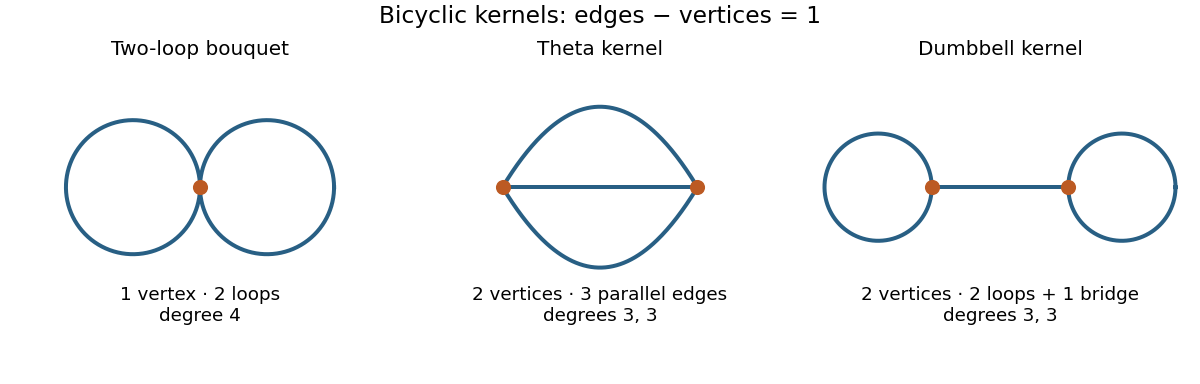
The two-loop bouquet, theta and dumbbell kernels of connected bicyclic graphs
. Details. 
Let count labelled bicyclic cores on a fixed -vertex set. The classification gives an absolute constant withTo see the bound concretely, order the one or two branching labels, choose one of the three kernel types, and distribute the other labels as ordered internal vertices of its two or three edges. There are at most weak compositions of their lengths, and at most ordered assignments of all labels. This overcounts orientations and edge permutations and ignores simplicity restrictions, both harmless for an upper bound.
For a lower bound, use only theta cores whose three paths each have at least one internal vertex. For , choose an ordered pair of branching vertices and an ordered list of the other labels, then cut that list into three nonempty ordered paths. There are encodings. Every resulting simple theta core is encoded exactly times, by swapping the branching vertices and permuting the three paths. Hence
Choose the core's vertices and attach the forest counted in part (i). The decomposition is unique, soPutting , the two estimates on reduce the labelled bicyclic graph count to the sum of divided by .
For the upper bound, givesThe corresponding sum is . For example, divide the positive integers into blocks : the sum in block is at most a constant times , and the series over converges. Including the finitely small indices makes no difference. Therefore .
For the lower bound, take sufficiently large and . Then , and throughout the product. Since on ,There are at least such integer indices, each with . The lower core bound therefore givesThis proves the two-sided bounds for all sufficiently large . They extend to every by adjusting the constants over the remaining finite set: there, since minus one edge is connected with five edges, and adding a pendant path supplies an example at every larger order. Consequently the correctly qualified conclusion isThe exceptional is a genuine defect in the printed quantifier, not a missing case of the proof.
Articles by others on the same topic
There are currently no matching articles.